Week 1: Math Bootcamp

RSM338: Machine Learning in Finance

Author

Kevin Mott

1 Introduction

In traditional programming, you write explicit rules for the computer to follow: “if the price drops 10%, sell.” You specify the logic. Machine learning is different. Instead of writing rules, you show the computer examples and let it discover patterns from the statistical properties of the data. The computer learns what predicts what.

Finance generates enormous amounts of data: prices, returns, fundamentals, news, filings, transactions. Machine learning gives us tools to extract information from all of it. Think of ML methods as tools in a toolbox—just as an experienced contractor knows which tool is right for each job, you’ll learn which ML method is right for each problem: regression for predicting continuous values like returns, classification for assigning categories like default/no-default, clustering for finding natural groupings, and text analysis for extracting information from documents.

Traditional finance models are elegant but limited. CAPM says expected returns depend on one factor (market beta); Fama-French adds size and value; but there are hundreds of potential predictors. Machine learning lets us handle many variables at once, capture nonlinear relationships, and let the data tell us what matters. The catch: finance is noisy, and patterns that look predictive often aren’t. A major theme of this course is learning to distinguish real signal from noise.

This chapter builds the mathematical foundation for everything that follows. We cover notation, key functions, and four main topics: statistics (random variables, distributions, expected value, variance), calculus (derivatives and how to find minima), linear algebra (vectors, matrices, and why they matter), and optimization (putting it together to find the best parameters). The goal is to increase your fluency reading mathematical expressions—we will NOT need to solve math problems by hand or complete any proofs.

2 Notation

Don’t panic when you see Greek letters—they’re just names for quantities. When you see $\mu$, think “the mean.” When you see $\sigma$, think “the standard deviation.” Here are the symbols you’ll encounter most often:

Symbol	Name	Common meaning
$\mu$	mu	Mean (expected value)
$\sigma$	sigma	Standard deviation
$\rho$	rho	Correlation
$\beta$	beta	Regression coefficient / market sensitivity
$\alpha$	alpha	Intercept / excess return
$\theta$	theta	Generic parameter
$\epsilon$	epsilon	Error term / noise
$\lambda$	lambda	Regularization parameter

Subscripts identify which observation or which variable we’re talking about. Time subscripts like $r_t$ denote the return at time $t$, while $P_{t-1}$ is the price one period earlier. Observation subscripts like $x_i$ and $y_i$ refer to the value for observation $i$. Variable subscripts like $\beta_j$ refer to the coefficient for feature $j$. We can combine them: $x_{ij}$ means feature $j$ for observation $i$.

The summation symbol $\Sigma$ (capital sigma) means “add up.” We read $\sum_{i=1}^{n} x_i = x_1 + x_2 + \cdots + x_n$ as “sum of $x_i$ from $i = 1$ to $n$.” The sample mean $\bar{x} = \frac{1}{n} \sum_{i=1}^{n} x_i$ and sample variance $\text{Var}(X) = \frac{1}{n-1} \sum_{i=1}^{n} (x_i - \bar{x})^2$ both use this notation. The product symbol $\Pi$ (capital pi) means “multiply together”: $\prod_{i=1}^{n} x_i = x_1 \times x_2 \times \cdots \times x_n$. This matters for finance because compounding returns multiply—if you earn returns $R_1, R_2, \ldots, R_T$ over $T$ periods, your wealth grows by $\prod_{t=1}^{T} (1 + R_t)$.

3 Logarithms and Exponentials

In finance, we constantly use log returns, so understanding logarithms is essential. The exponential function $e^x$ (where $e \approx 2.718$) and the natural logarithm $\ln(x)$ are inverses of each other: $\ln(e^x) = x$ and $e^{\ln(x)} = x$.

Logarithms have three key properties that make them useful: they turn multiplication into addition ($\ln(a \times b) = \ln(a) + \ln(b)$), division into subtraction ($\ln(a / b) = \ln(a) - \ln(b)$), and exponents into multiplication ($\ln(a^b) = b \cdot \ln(a)$).

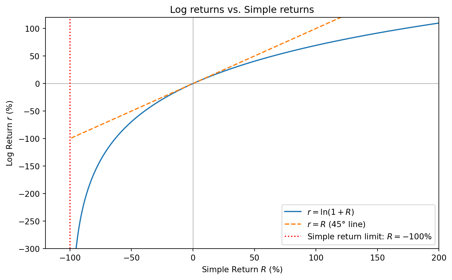
Instead of the simple return $R_t = \frac{P_t - P_{t-1}}{P_{t-1}}$, we often use the log return: \[r_t = \ln(1+R_t) = \ln\left(\frac{P_t}{P_{t-1}}\right) = \ln(P_t) - \ln(P_{t-1})\]

Why log returns are better:

Additivity: Multi-period log returns just add up: $r_{1 \to T} = r_1 + r_2 + \cdots + r_T$
Symmetry: A +50% log return followed by -50% log return gets you back to start. With simple returns, a -50% loss requires a +100% gain to recover!
Unboundedness: Simple returns are bounded below at -100% (you can’t lose more than everything). Log returns range from $-\infty$ to $+\infty$, which is better for statistical modeling.
Normality: Log returns are closer to normally distributed than simple returns.

For small returns, log and simple returns are nearly identical (they both follow the 45° line near the origin). But they diverge for large movements: log returns compress large gains and stretch large losses. As simple returns approach -100%, log returns go to $-\infty$—the log transform “knows” that losing everything is infinitely bad.

import numpy as np

# Computing log returns from prices
prices = np.array([100, 105, 102, 108, 110])
log_returns = np.log(prices[1:]) - np.log(prices[:-1])

print(f"Prices: {prices}")
print(f"Log returns: {log_returns}")
print(f"Sum of log returns: {log_returns.sum():.4f}")
print(f"ln(final/initial): {np.log(prices[-1]/prices[0]):.4f}")  # Same!

Prices: [100 105 102 108 110]
Log returns: [ 0.04879016 -0.02898754  0.05715841  0.01834914]
Sum of log returns: 0.0953
ln(final/initial): 0.0953

4 Statistics

4.1 Random Variables and Distributions

A random variable is a quantity whose value is determined by chance—tomorrow’s S&P 500 return, the outcome of rolling a die, whether a borrower defaults. We use capital letters like $X$, $Y$, $R$ for random variables; when we write $X = 3$, we mean “the random variable $X$ takes the value 3.”

We can’t predict the exact value of a random variable, but we often have historical data—past realizations of the same random process. By looking at many past realizations, we can see patterns: some outcomes happen frequently, others are rare. This pattern of “how likely is each outcome?” is called a distribution. When we write $X \sim \text{Distribution}$, we’re saying the random variable $X$ follows this pattern.

import matplotlib.pyplot as plt

np.random.seed(42)
sample_sizes = [100, 1000, 10000, 100000, 1000000]

fig, axes = plt.subplots(1, 5, figsize=(15, 3), sharey=True)
for ax, n in zip(axes, sample_sizes):
    rolls = np.random.randint(1, 7, size=n)
    values, counts = np.unique(rolls, return_counts=True)
    ax.bar(values, counts / n)
    ax.axhline(1/6, color='red', linestyle='--')
    ax.set_title(f'n = {n:,}')
    ax.set_xlabel('$X$')
axes[0].set_ylabel('$p(X)$')
plt.tight_layout()
plt.show()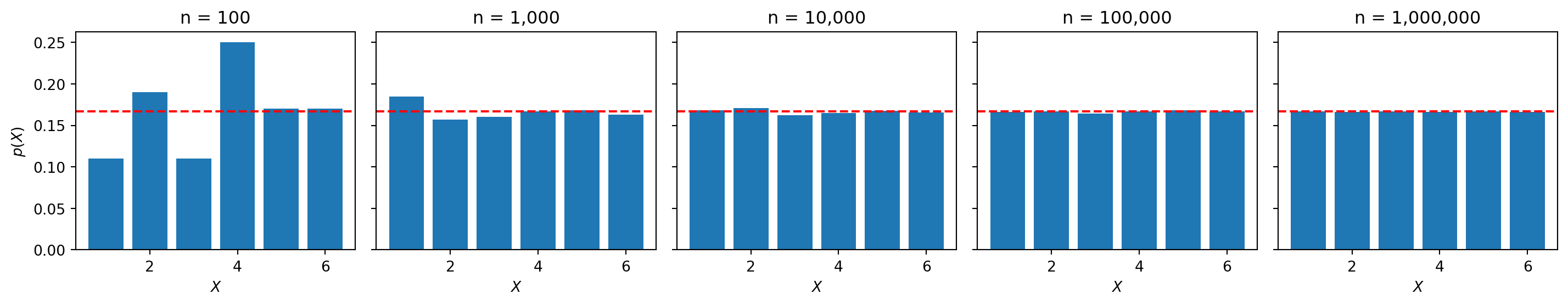

With only 100 rolls, the pattern is noisy. With a million rolls, it’s nearly perfect—each value appears almost exactly 1/6 of the time (red dashed line). More data gives us a clearer picture of the true distribution. This is a uniform distribution: each outcome is equally likely.

4.2 Common Distributions

The normal distribution (or Gaussian) is the “bell curve”—most values cluster near the center, with extreme values increasingly rare. We write $X \sim \mathcal{N}(\mu, \sigma^2)$ where $\mu$ is the mean (center) and $\sigma$ is the standard deviation (spread).

from scipy.stats import norm

np.random.seed(42)
x_grid = np.linspace(-4, 4, 100)

fig, axes = plt.subplots(1, 5, figsize=(15, 3), sharey=True)
for ax, n in zip(axes, sample_sizes):
    samples = np.random.normal(loc=0, scale=1, size=n)
    ax.hist(samples, bins=30, density=True)
    ax.plot(x_grid, norm.pdf(x_grid), color='red', linestyle='--')
    ax.set_title(f'n = {n:,}')
    ax.set_xlabel('$X$')
axes[0].set_ylabel('$p(X)$')
plt.tight_layout()
plt.show()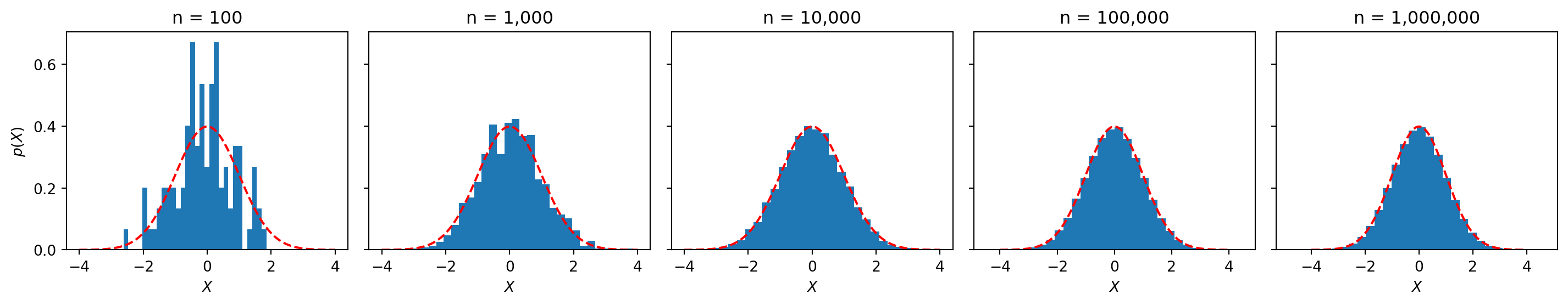

The Bernoulli distribution models yes/no outcomes: something happens (1) or doesn’t (0). We write $X \sim \text{Bernoulli}(p)$ where $p$ is the probability of success. Finance examples include whether a borrower defaults, whether a stock beats the market, or whether a transaction is fraudulent.

The normal distribution shows up everywhere because of the central limit theorem: no matter what the underlying distribution looks like, the distribution of sample means becomes a bell curve as sample size increases. The CLT tells us $\bar{X} \sim \mathcal{N}(\mu, \sigma^2/n)$—the spread of our estimates shrinks like $\sigma / \sqrt{n}$. To cut your estimation error in half, you need four times as much data.

Discrete distributions have $X$ taking a finite set of values (die rolls, loan defaults), while continuous distributions have $X$ taking any value in a range (stock returns, interest rates).

4.3 Expected Value and Variance

The expected value $\mathbb{E}[X]$ (also written $\mu$) is the probability-weighted average of all possible outcomes: \[\mathbb{E}[X] = \sum_{i=1}^{k} x_i \cdot p(x_i)\] Each outcome is weighted by how likely it is—outcomes that happen often contribute more. From samples, we estimate it with the sample mean $\bar{x} = \frac{1}{n}\sum_{i=1}^{n} x_i$. Outliers distort the mean because even rare events (low $p(x_i)$) can contribute heavily if $x_i$ is extreme.

Variance $\text{Var}(X) = \sigma^2$ measures how spread out values are around the mean: \[\text{Var}(X) = \mathbb{E}[(X - \mu)^2] = \sum_{i=1}^{k} (x_i - \mu)^2 \cdot p(x_i)\] The standard deviation $\sigma = \sqrt{\text{Var}(X)}$ is in the same units as $X$. From samples, we estimate variance with $s^2 = \frac{1}{n-1}\sum_{i=1}^{n}(x_i - \bar{x})^2$. In finance, standard deviation of returns is called volatility.

4.4 Covariance, Correlation, and Regression

Covariance measures whether two variables move together: $\text{Cov}(X, Y) = \mathbb{E}[(X - \mu_X)(Y - \mu_Y)]$. Positive covariance means when $X$ is high, $Y$ tends to be high; negative means they move opposite. Correlation scales covariance to $[-1, 1]$: \[\rho_{XY} = \frac{\text{Cov}(X, Y)}{\sigma_X \cdot \sigma_Y}\] A correlation of $+1$ means perfect positive relationship, $0$ means no linear relationship, and $-1$ means perfect negative relationship. In portfolio theory, diversification works because assets with low or negative correlation reduce portfolio variance.

Linear regression goes further than correlation—it finds the best-fitting line $Y = \alpha + \beta X + \epsilon$, where $\alpha$ is the intercept, $\beta$ is the slope (how much $Y$ changes when $X$ increases by 1), and $\epsilon$ is the error term. The sign of $\beta$ matches the sign of correlation.

from sklearn.linear_model import LinearRegression

np.random.seed(42)
market = np.random.normal(0, 0.02, 100)
stock = 1.2 * market + np.random.normal(0, 0.01, 100)

model = LinearRegression()
model.fit(market.reshape(-1, 1), stock)

print(f"Intercept (alpha): {model.intercept_:.4f}")
print(f"Slope (beta): {model.coef_[0]:.4f}")
print(f"Correlation: {np.corrcoef(market, stock)[0,1]:.4f}")

plt.scatter(market, stock)
plt.plot(market, model.predict(market.reshape(-1, 1)), color='red', label=f'beta = {model.coef_[0]:.2f}')
plt.xlabel('Market return ($X$)')
plt.ylabel('Stock return ($Y$)')
plt.legend()
plt.show()

Intercept (alpha): 0.0001
Slope (beta): 1.1284
Correlation: 0.9082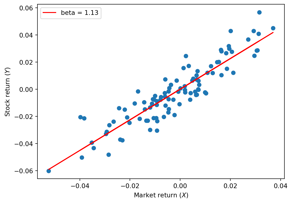

This is the foundation of machine learning: finding relationships in data. sklearn (scikit-learn) is the library we’ll use throughout this course.

5 Calculus

5.1 Functions and Derivatives

A function takes an input and produces an output: for $f(x) = x^2$, input $x = 3$ gives output $f(3) = 9$. In ML, we work with functions that measure error and want to find the input that makes error as small as possible.

For a straight line, the slope tells you how steep it is: $\text{slope} = \frac{\Delta y}{\Delta x}$. Positive slope means the line goes up as you move right; negative means it goes down; zero means flat. But for curves, the slope is different at every point.

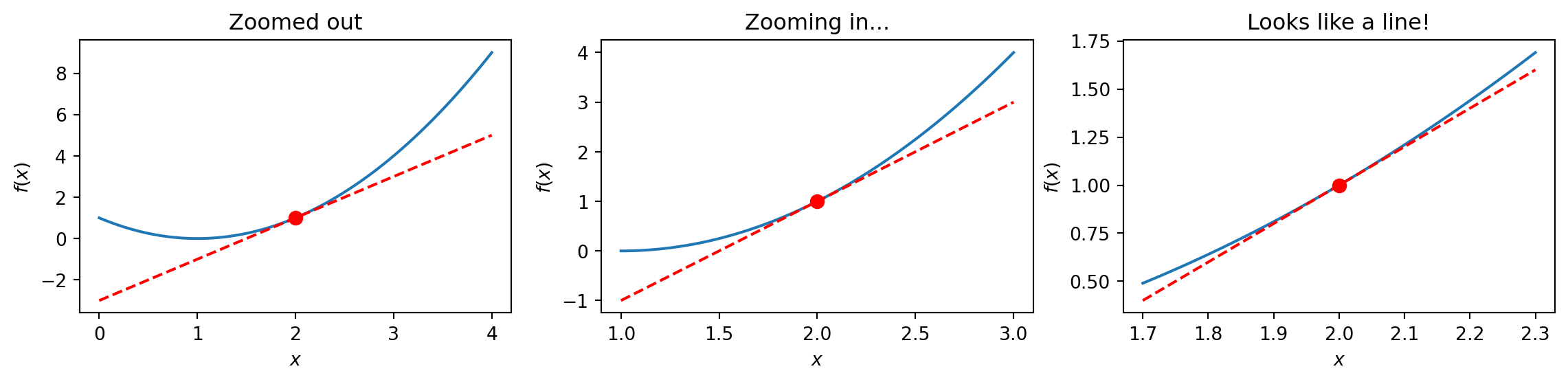
The derivative $f'(x)$ is the slope of a curve at a specific point—the “instantaneous” rate of change. Imagine zooming in on a curve until it looks like a straight line; the slope of that line is the derivative. Several notations mean the same thing: $f'(x) = \frac{df}{dx} = \frac{d}{dx}f(x)$. What the derivative tells you: $f'(x) > 0$ means the function is increasing at $x$; $f'(x) < 0$ means decreasing; $f'(x) = 0$ means flat.

5.2 Finding Minima

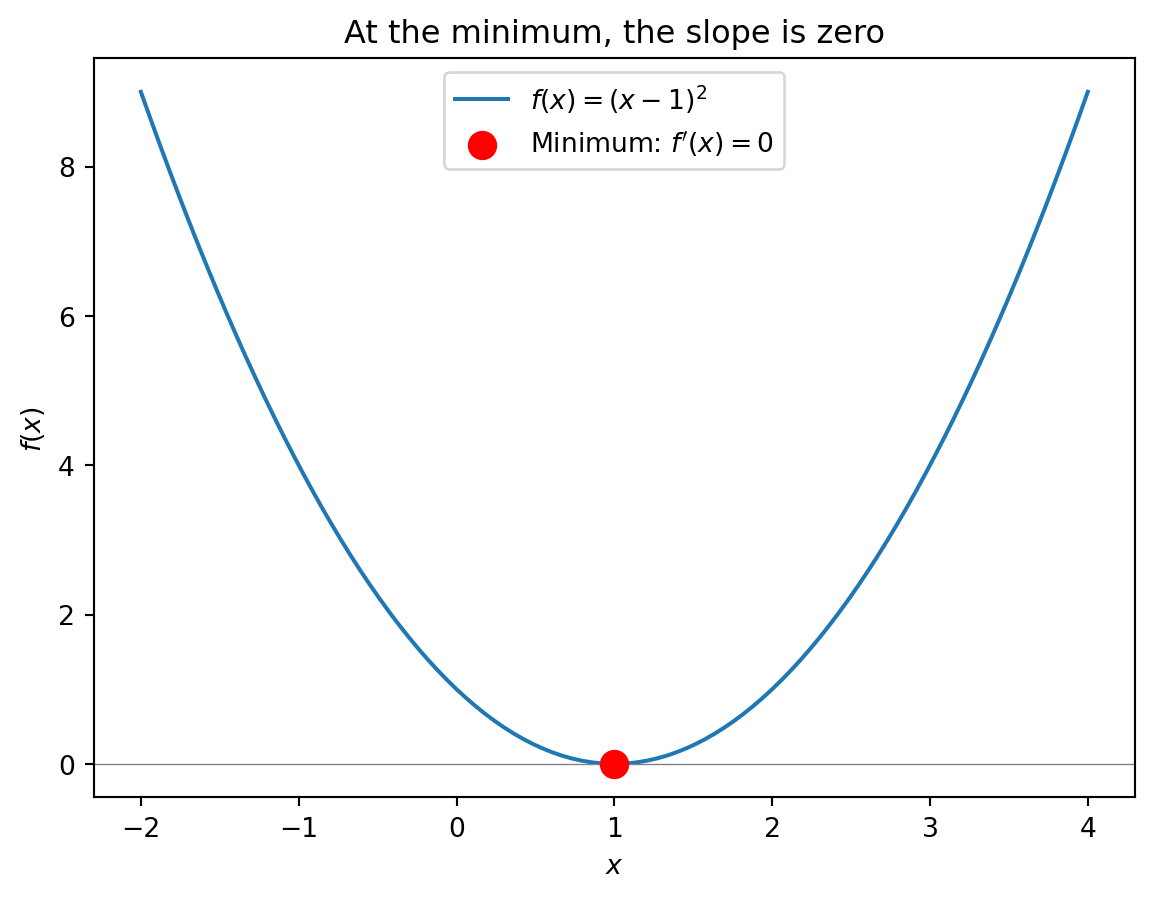
An extremum is a minimum or maximum of a function. At an extremum, the function is flat—it’s neither increasing nor decreasing, so the derivative is zero. To find the minimum of $f(x)$: take the derivative $f'(x)$, set $f'(x) = 0$, and solve for $x$. You won’t compute derivatives by hand in this course—computers handle that—but you need to understand the logic: the minimum is where the slope is zero.

5.3 Functions of Multiple Variables

So far we’ve looked at functions of one variable: $f(x)$. But what if a function depends on two (or more) variables? Consider: \[f(x_1, x_2) = -(x_1^2 + x_2^2)\]

This function takes two inputs and produces one output. We can visualize it as a surface in 3D:

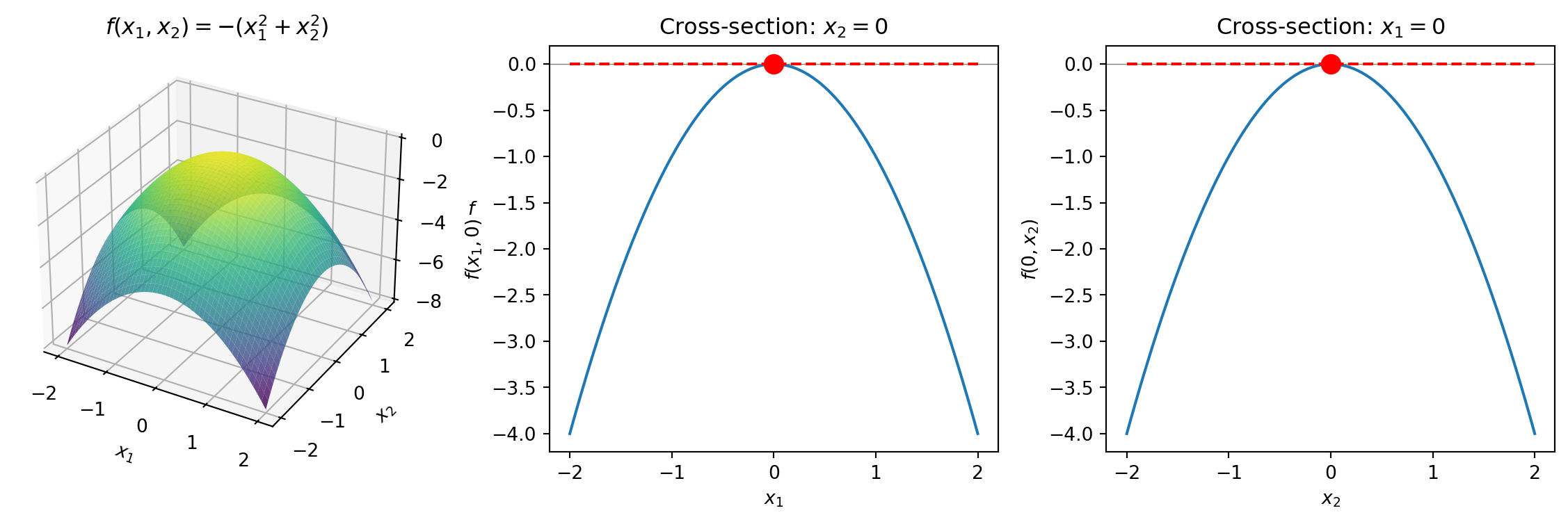
The maximum is at the origin $(0, 0)$—the top of the “dome.” In both cross-sections, the tangent line is flat (slope = 0) at the extremum.

5.4 Partial Derivatives

How do we find the extremum of a function with multiple variables? We ask: if I move in just the $x_1$ direction (holding $x_2$ fixed), what’s the slope? That’s the partial derivative with respect to $x_1$. We write it as $\frac{\partial f}{\partial x_1}$.

Look back at our cross-sections: each one shows the slope in one direction. At the top of the dome, both cross-sections are flat—the slope is zero in every direction.

At an extremum, all partial derivatives are zero. The surface is flat no matter which direction you look. This is what optimization algorithms search for.

Why this matters for ML: We define a loss function that measures error. Training a model means finding parameters that minimize that loss—finding where all the partial derivatives are zero.

6 Linear Algebra

6.1 Vectors and Matrices

Linear relationships are easy to work with: easy to compute, easy to optimize, easy to interpret. Vectors and matrices let us extend these relationships to multiple dimensions.

A vector $\mathbf{x}$ is an ordered list of numbers. We write vectors as columns: \[\mathbf{x} = \begin{bmatrix} x_1 \\ x_2 \\ \vdots \\ x_n \end{bmatrix} \in \mathbb{R}^n\] The notation $\mathbf{x} \in \mathbb{R}^n$ means “$\mathbf{x}$ has $n$ real numbers.”

A matrix $\mathbf{X}$ is a 2D array of numbers arranged in rows and columns: \[\mathbf{X} = \begin{bmatrix} x_{11} & x_{12} & \cdots & x_{1p} \\ x_{21} & x_{22} & \cdots & x_{2p} \\ \vdots & \vdots & \ddots & \vdots \\ x_{n1} & x_{n2} & \cdots & x_{np} \end{bmatrix} \in \mathbb{R}^{n \times p}\] This matrix has $n$ rows (observations) and $p$ columns (features). Element $x_{ij}$ is in row $i$, column $j$.

x = np.array([1, 2, 3, 4, 5])
print(f"Vector x = {x}, has {len(x)} elements")

X = np.array([[1, 2, 3], [4, 5, 6]])
print(f"\nMatrix X has shape {X.shape}:\n{X}")

Vector x = [1 2 3 4 5], has 5 elements

Matrix X has shape (2, 3):
[[1 2 3]
 [4 5 6]]

The transpose $\mathbf{X}'$ (or $\mathbf{X}^T$) flips rows and columns. An $(n \times p)$ matrix becomes $(p \times n)$: \[\mathbf{X} = \begin{bmatrix} 1 & 2 & 3 \\ 4 & 5 & 6 \end{bmatrix} \quad \Rightarrow \quad \mathbf{X}' = \begin{bmatrix} 1 & 4 \\ 2 & 5 \\ 3 & 6 \end{bmatrix}\] In Python, use .T for transpose.

To multiply matrices $\mathbf{A}$ and $\mathbf{B}$, the inner dimensions must match: $(m \times n) \cdot (n \times p) = (m \times p)$. The result has the same number of rows as $\mathbf{A}$ and columns as $\mathbf{B}$. Each element of the output is a dot product: element $(i,j)$ of $\mathbf{C} = \mathbf{A}\mathbf{B}$ is $C_{ij} = \sum_k A_{ik} B_{kj}$—row $i$ of $\mathbf{A}$ dotted with column $j$ of $\mathbf{B}$.

Advanced: How Matrix Multiplication Works

To compute $\mathbf{C} = \mathbf{A} \mathbf{B}$, element $C_{ij}$ is the dot product of row $i$ of $\mathbf{A}$ with column $j$ of $\mathbf{B}$: \[\begin{bmatrix} \colorbox{yellow}{$a$} & \colorbox{yellow}{$b$} \\ c & d \end{bmatrix} \begin{bmatrix} e & \colorbox{yellow}{$f$} \\ g & \colorbox{yellow}{$h$} \end{bmatrix} = \begin{bmatrix} ae+bg & \colorbox{yellow}{$af+bh$} \\ ce+dg & cf+dh \end{bmatrix}\] The highlighted element $(1,2)$ comes from row 1 of $\mathbf{A}$ (highlighted) dotted with column 2 of $\mathbf{B}$ (highlighted): $a \cdot f + b \cdot h$.

In Python, use @ for matrix multiplication and .T for transpose:

C = A @ B    # matrix multiplication
A_transpose = A.T    # transpose

A = np.array([[1, 2], [3, 4]])
B = np.array([[5, 6], [7, 8]])
C = A @ B  # @ is matrix multiplication
print(f"A @ B =\n{C}")
print(f"\nC[0,1] = 1*6 + 2*8 = {C[0,1]}")
print(f"\nA.T =\n{A.T}")

A @ B =
[[19 22]
 [43 50]]

C[0,1] = 1*6 + 2*8 = 22

A.T =
[[1 3]
 [2 4]]

Warning

Matrix multiplication is NOT commutative: $\mathbf{A}\mathbf{B} \neq \mathbf{B}\mathbf{A}$ in general. The order matters!

The identity matrix $\mathbf{I}$ has 1s on the diagonal and 0s elsewhere: \[\mathbf{I} = \begin{bmatrix} 1 & 0 & \cdots & 0 \\ 0 & 1 & \cdots & 0 \\ \vdots & \vdots & \ddots & \vdots \\ 0 & 0 & \cdots & 1 \end{bmatrix}\] It satisfies $\mathbf{A}\mathbf{I} = \mathbf{I}\mathbf{A} = \mathbf{A}$. The inverse $\mathbf{A}^{-1}$ satisfies $\mathbf{A}^{-1}\mathbf{A} = \mathbf{I}$, letting us “undo” multiplication.

6.2 Application: OLS in Matrix Form

In linear regression, we want to predict $y$ from multiple variables $x_1, x_2, \ldots, x_p$: \[y = \beta_0 + \beta_1 x_1 + \beta_2 x_2 + \cdots + \beta_p x_p + \epsilon\]

But we have $n$ observations, so we need $n$ equations: \[\begin{align*} y_1 &= \beta_0 + \beta_1 x_{11} + \beta_2 x_{12} + \cdots + \beta_p x_{1p} + \epsilon_1 \\ y_2 &= \beta_0 + \beta_1 x_{21} + \beta_2 x_{22} + \cdots + \beta_p x_{2p} + \epsilon_2 \\ &\vdots \\ y_n &= \beta_0 + \beta_1 x_{n1} + \beta_2 x_{n2} + \cdots + \beta_p x_{np} + \epsilon_n \end{align*}\]

Stack everything into vectors and matrices: \[\underbrace{\mathbf{y}}_{n \times 1} = \underbrace{\mathbf{X}}_{n \times p} \underbrace{\boldsymbol{\beta}}_{p \times 1} + \underbrace{\boldsymbol{\epsilon}}_{n \times 1}\]

The ordinary least squares (OLS) solution is: $\hat{\boldsymbol{\beta}} = (\mathbf{X}'\mathbf{X})^{-1}\mathbf{X}'\mathbf{y}$

Advanced: Where does the OLS formula come from?

Start with $\mathbf{y} = \mathbf{X}\boldsymbol{\beta} + \boldsymbol{\epsilon}$. In expectation, $\boldsymbol{\epsilon}$ averages to zero, so we want to solve $\mathbf{y} = \mathbf{X}\boldsymbol{\beta}$ for $\boldsymbol{\beta}$.

We’d like to “divide by $\mathbf{X}$” but $\mathbf{X}$ is $(n \times p)$—not square, so not invertible!

The trick: premultiply both sides by $\mathbf{X}'$ to make it square: \[\mathbf{X}'\mathbf{y} = \mathbf{X}'\mathbf{X}\boldsymbol{\beta}\]

Now $\mathbf{X}'\mathbf{X}$ is $(p \times p)$—square and invertible. Premultiply both sides by $(\mathbf{X}'\mathbf{X})^{-1}$: \[\begin{align*} (\mathbf{X}'\mathbf{X})^{-1}\mathbf{X}'\mathbf{y} &= (\mathbf{X}'\mathbf{X})^{-1}\mathbf{X}'\mathbf{X}\boldsymbol{\beta} \\ (\mathbf{X}'\mathbf{X})^{-1}\mathbf{X}'\mathbf{y} &= \mathbf{I}\boldsymbol{\beta} \\ \boldsymbol{\beta} &= (\mathbf{X}'\mathbf{X})^{-1}\mathbf{X}'\mathbf{y} \end{align*}\]

6.3 The Gradient

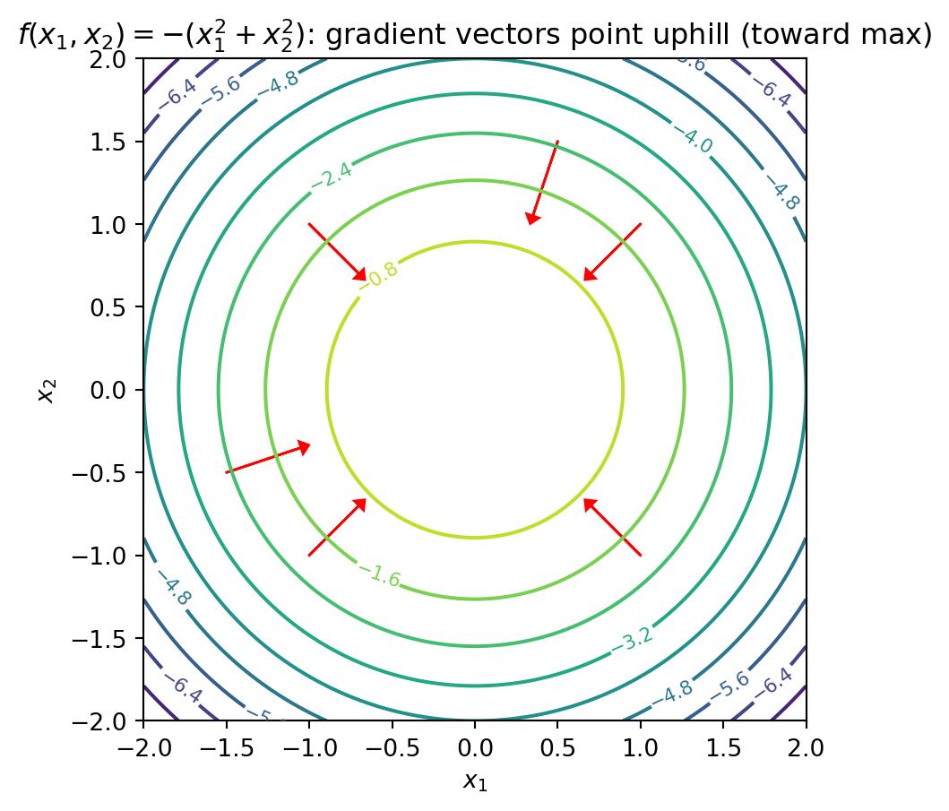
The gradient is the vector of all partial derivatives: \[\nabla f = \begin{bmatrix} \frac{\partial f}{\partial x_1} \\ \frac{\partial f}{\partial x_2} \\ \vdots \\ \frac{\partial f}{\partial x_p} \end{bmatrix}\]

Since the gradient is a vector, it points in a direction. Which direction? The direction of steepest increase. To find a minimum: follow $-\nabla f$ (the direction of steepest decrease).

7 Optimization

When we write $\boldsymbol{\theta}^* = \arg\min_{\boldsymbol{\theta}} \mathcal{L}(\boldsymbol{\theta})$, we mean “$\boldsymbol{\theta}^*$ is the value that minimizes $\mathcal{L}$.” Note: $\min$ gives you the minimum value, while $\arg\min$ gives you the input that achieves it.

Machine learning is optimization. Given data $(\mathbf{X}, \mathbf{y})$, we find parameters $\boldsymbol{\theta}$ that minimize a loss function: \[\boldsymbol{\theta}^* = \arg\min_{\boldsymbol{\theta}} \mathcal{L}(\boldsymbol{\theta}; \mathbf{X}, \mathbf{y})\]

For linear regression, the loss function is $\mathcal{L}(\boldsymbol{\beta}) = \sum_{i=1}^n (y_i - \mathbf{x}_i'\boldsymbol{\beta})^2$ and the solution is the OLS formula.

Advanced: Closed-Form Solutions vs. Algorithms

OLS has a nice closed-form solution: we can write down a formula $\hat{\boldsymbol{\beta}} = (\mathbf{X}'\mathbf{X})^{-1}\mathbf{X}'\mathbf{y}$ and compute the answer directly.

Most ML methods don’t have this luxury. For neural networks, random forests, and many other models, there’s no formula—we have to search for the optimum iteratively using algorithms like gradient descent: start somewhere, compute the gradient, take a step downhill, repeat.

That’s why we spend so much time on optimization in this course: understanding how these algorithms work is essential for understanding modern machine learning.

Everything in this chapter is a building block: statistics tells us what we’re estimating, calculus tells us how to find minima, linear algebra gives us compact notation, and optimization ties it all together.

8 Appendix: Setting Up Python

Install VS Code from code.visualstudio.com—it’s a free, lightweight editor that works on all platforms.

Install Python from python.org/downloads. On Windows, check “Add Python to PATH” during installation. On Mac, you can also use Homebrew: brew install python.

Install the Python extension in VS Code: click Extensions in the left sidebar, search “Python”, and install the Microsoft extension.

Install packages by opening a terminal and running:

pip install numpy pandas matplotlib scikit-learn

Verify your setup by creating test_setup.py:

import numpy as np
import pandas as pd
import matplotlib.pyplot as plt
from sklearn.linear_model import LinearRegression
print("All packages imported successfully!")

If you see “All packages imported successfully!” you’re ready to go. If you run into issues, office hours are a good time to troubleshoot.

Week 2: Financial Data I