Much of quantitative finance—and the machine learning applications we will study—centers on return prediction. We model and forecast returns because they have convenient statistical properties: they’re stationary (roughly the same distribution over time), they aggregate nicely across assets, and they’re what most financial theories are built around. The Capital Asset Pricing Model, the Fama-French factor models, mean-variance optimization—all of these work with returns.
However, investors ultimately care about wealth: the dollar value of their portfolio. If you’re saving for retirement, you want to know how much money you’ll have in 30 years, not what your average annual return will be. And here’s the problem: wealth is a nonlinear function of returns. In general, for a nonlinear function \(f\) and random variable \(X\), the expected value \(\mathbb{E}[f(X)] \neq f(\mathbb{E}[X])\). This seemingly technical point has profound practical implications. It means that knowing the expected return does not directly tell us the expected wealth. And as we’ll see, the gap between these two quantities can be enormous over long time horizons.
This chapter develops the statistical framework for working with financial returns. We start with the definitions of simple and log returns, explaining why quantitative finance has converged on log returns as the standard working unit. We then explore what happens when we assume log returns are normally distributed—a foundational assumption in finance. That assumption implies wealth follows a log-normal distribution, which has surprising consequences for expected values: most investors will end up with less than the “expected” wealth, because the mean is pulled up by a small number of extremely lucky outcomes.
We then examine estimation risk—the additional uncertainty that arises because we must estimate parameters from historical data rather than knowing them with certainty. This adds another layer of upward bias to wealth forecasts. Finally, we test whether the normality assumption actually holds in practice (spoiler: not perfectly—real returns have “fat tails” that make extreme events far more common than normal predicts) and preview why prediction is so difficult in finance.
2 Returns
2.1 Simple Returns
The simple return (or arithmetic return) from period \(t-1\) to \(t\) measures the percentage change in value: \[R_t = \frac{P_t + d_t}{P_{t-1}} - 1\] where \(P_t\) is the price at time \(t\), \(P_{t-1}\) is the price at time \(t-1\), and \(d_t\) is any dividend paid during the period. If you invest $100, the stock rises to $105, and you receive a $2 dividend, your simple return is \((105 + 2)/100 - 1 = 7\%\).
Simple returns have an intuitive interpretation: they tell you directly how much your wealth grew in percentage terms. If your portfolio was worth $10,000 and you earned a 7% simple return, your portfolio is now worth $10,700. This directness makes simple returns the natural choice for communicating performance to clients or comparing across investments.
But simple returns have an inconvenient property when we compound over multiple periods, and this inconvenience matters enormously for statistical analysis.
2.2 The Problem with Simple Returns
Suppose you earn \(R_1 = 10\%\) in year 1 and \(R_2 = 10\%\) in year 2. Your total return over both years is not\(10\% + 10\% = 20\%\). Instead: \[1 + R_{1\to2} = (1 + R_1)(1 + R_2) = (1.10)(1.10) = 1.21\] So \(R_{1\to2} = 21\%\). Simple returns compound multiplicatively, not additively. In general, over \(T\) years: \[1 + R_{1 \to T} = \prod_{t=1}^{T} (1 + R_t)\]
This multiplicative structure makes simple returns awkward for statistical analysis. If we want to annualize a multi-year return, we need to take a \(T\)-th root: \(\bar{R} = (1 + R_{1 \to T})^{1/T} - 1\). But this is a nonlinear function of returns, and recall from Week 1 that \(\mathbb{E}[f(X)] \neq f(\mathbb{E}[X])\) for nonlinear \(f\). This means the expected annualized return is not the annualized expected return—a confusing situation. Variances don’t scale nicely either: the variance of a 10-year return is not simply 10 times the variance of a 1-year return.
These complications make it difficult to build statistical models with simple returns. We need a transformation that converts multiplication into addition—and fortunately, that’s exactly what logarithms do.
2.3 Log Returns
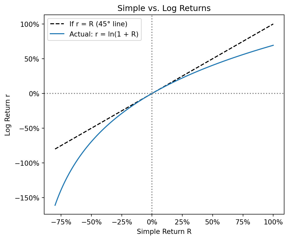
Given a simple return \(R\), the log return (or continuously compounded return) \(r\) is defined by: \[e^r = 1 + R \quad \Longleftrightarrow \quad r = \ln(1 + R)\]
For stocks, the gross return is \(1 + R_t = P_t / P_{t-1}\), so: \[r_t = \ln\left(\frac{P_t}{P_{t-1}}\right) = \ln(P_t) - \ln(P_{t-1})\]
Log returns are just differences in log prices—extremely convenient for computation.
The key advantage comes from the logarithm’s property that \(\ln(ab) = \ln(a) + \ln(b)\). Applied to multi-period returns: \[\begin{align*}
r_{1 \to T} &= \ln(1 + R_{1 \to T}) = \ln\left[\prod_{t=1}^{T}(1+R_t)\right] \\
&= \ln(1+R_1) + \ln(1+R_2) + \cdots + \ln(1+R_T) \\
&= r_1 + r_2 + \cdots + r_T = \sum_{t=1}^{T} r_t
\end{align*}\]
Log returns add over time. This is the key property that makes log returns so useful for statistical modeling. The annualized log return is simply the arithmetic mean: \(\bar{r} = r_{1 \to T} / T\). No roots, no messy exponents. This means all the machinery of statistics—means, variances, regressions, hypothesis tests—works cleanly with log returns. If you’ve taken a statistics course, everything you learned about sums of random variables applies directly.
import numpy as np# Simple returns for three yearsR = np.array([0.10, -0.05, 0.15])# Log returnsr = np.log(1+ R)print("Simple returns:", R)print("Log returns:", r.round(4))print(f"\nCumulative simple return: {np.prod(1+ R) -1:.4f}")print(f"Sum of log returns: {r.sum():.4f}")print(f"These match: exp({r.sum():.4f}) - 1 = {np.exp(r.sum()) -1:.4f}")
Simple returns: [ 0.1  -0.05  0.15]
Log returns: [ 0.0953 -0.0513  0.1398]

Cumulative simple return: 0.2017
Sum of log returns: 0.1838
These match: exp(0.1838) - 1 = 0.2017
For small returns, \(r_t \approx R_t\) because \(\ln(1+x) \approx x\) for small \(x\). The difference grows for larger returns. Note the asymmetry: a 50% simple gain gives \(r = \ln(1.5) = 40.5\%\), while a 50% simple loss gives \(r = \ln(0.5) = -69.3\%\).
Statistical convenience: Sums of random variables are easier to analyze than products
No lower bound: Log returns range from \(-\infty\) to \(+\infty\); simple returns are bounded below by \(-100\%\)
Normality: Log returns are closer to normally distributed than simple returns
Simple returns are what you actually earn. Log returns are what you compute with. We move between them as needed.
3 The Log-Normal Distribution of Wealth
3.1 The Key Assumption
A foundational assumption in quantitative finance is that log returns are normally distributed: \[r_t \sim N(\mu, \sigma^2)\]
This says each period’s log return is a random draw from a normal distribution with mean \(\mu\) (the expected log return) and variance \(\sigma^2\) (with \(\sigma\) being the volatility). Why is this assumption so common? First, empirical evidence suggests it’s a reasonable approximation for daily or monthly returns (though not perfect, as we’ll see later). Second, the normal distribution is mathematically tractable: we can derive closed-form expressions for expected values, variances, and probabilities. Third, the Central Limit Theorem tells us that sums of many small, independent effects tend toward normality—and stock returns arguably reflect the aggregation of many traders’ decisions.
But here’s where things get interesting. We don’t actually care about log returns—we care about wealth. If log returns are normally distributed, what does that imply for the distribution of wealth itself?
3.2 From Log Returns to Wealth
Suppose you start with wealth \(W_0\) and invest for \(T\) years. Your terminal wealth is the product of gross returns: \[W_T = W_0 \cdot (1 + R_1)(1 + R_2) \cdots (1 + R_T)\]
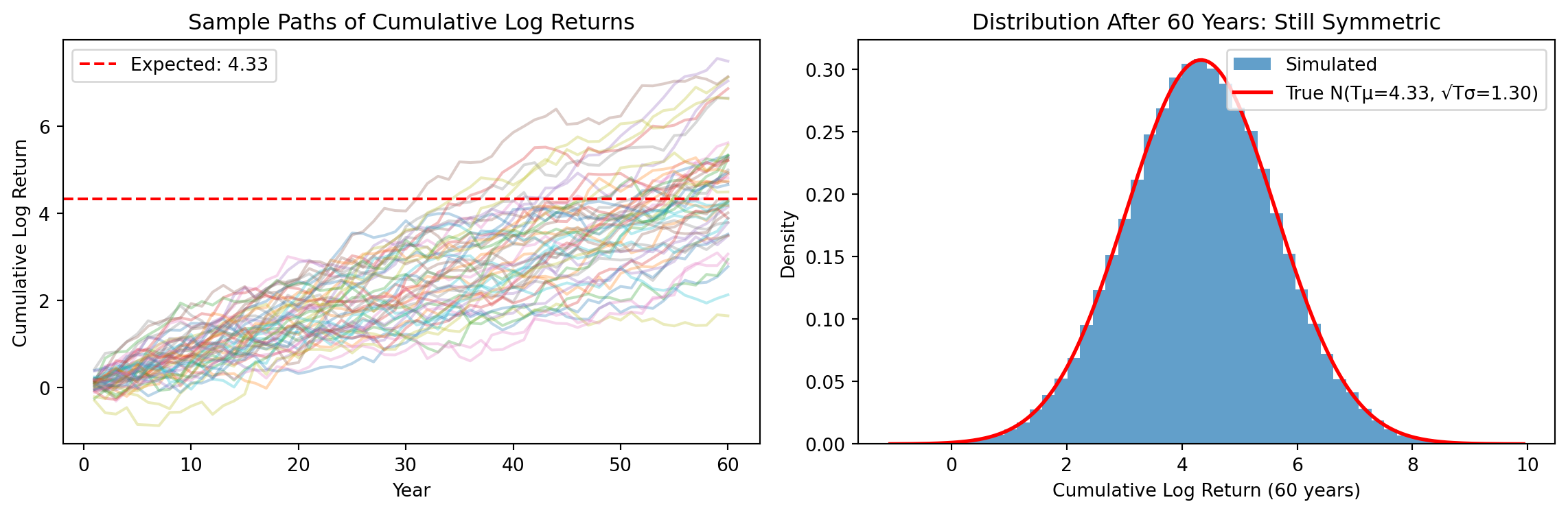
Log wealth growth is a sum of log returns. If each year’s log return is an independent draw from \(N(\mu, \sigma^2)\), then the sum of \(T\) such draws is: \[\sum_{t=1}^{T} r_t \sim N(T\mu, T\sigma^2)\]
Both the mean and variance scale with \(T\): expected cumulative return is \(T\mu\), and standard deviation grows with \(\sqrt{T}\).
3.3 The Log-Normal Distribution
Since \(\ln(W_T) = \ln(W_0) + \sum_{t=1}^{T} r_t\) and the sum is normal, we have: \[\ln(W_T) \sim N(\ln(W_0) + T\mu, T\sigma^2)\]
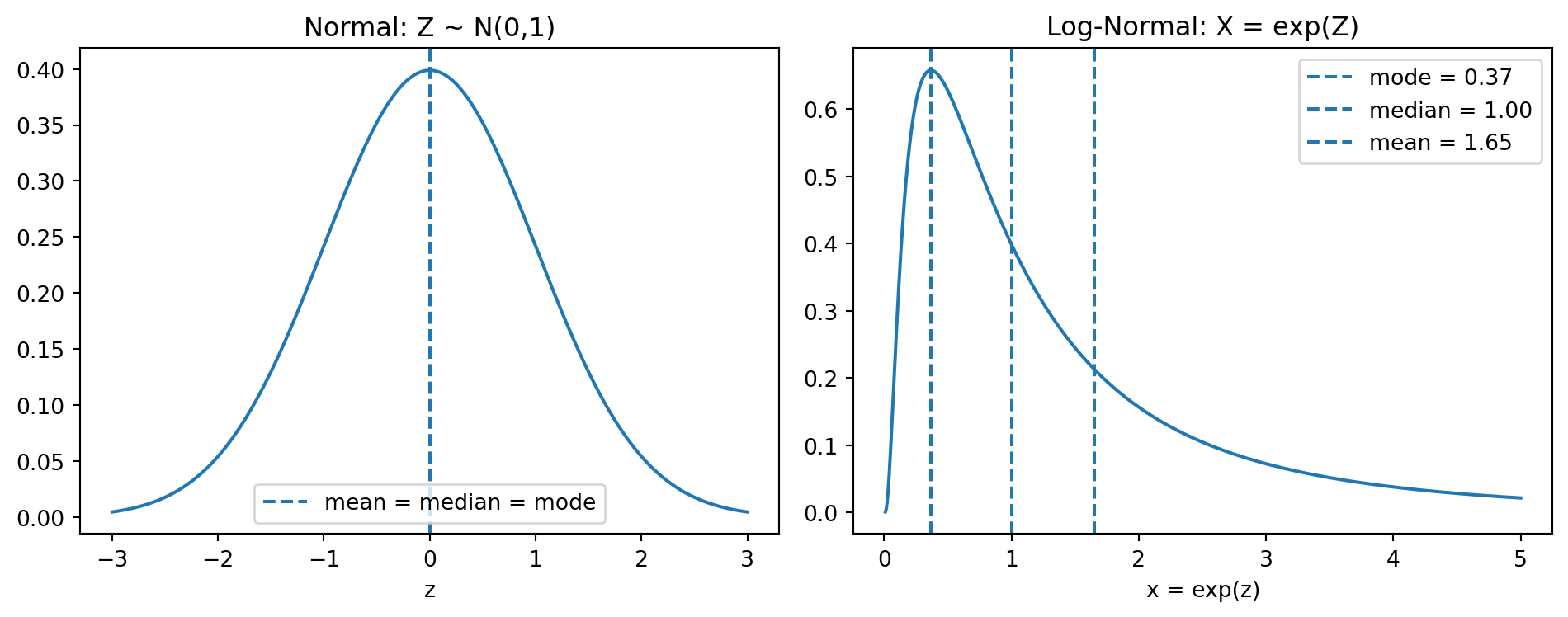
A random variable \(X\) is log-normally distributed if \(\ln(X)\) is normally distributed. Therefore:
Exponentiating a symmetric distribution creates asymmetry. For a log-normal distribution, Mode \(<\) Median \(<\) Mean.
3.4 The Variance Boost
We want to forecast expected terminal wealth \(\mathbb{E}[W_T]\). A tempting guess is \(\mathbb{E}[W_T] = W_0 \cdot e^{T\mu}\), plugging the expected cumulative log return into the exponential. This is what you’d get if returns were certain to equal their expected value every year. But returns are random, and this randomness matters.
The tempting guess implicitly assumes \(\mathbb{E}[e^Z] = e^{\mathbb{E}[Z]}\)—that the expected value of the exponential equals the exponential of the expected value. But this is false for nonlinear functions. The correct formula for the expected value of a log-normal is:
The variance appears in the expected value! This is remarkable: even if you know the mean of \(Z\) perfectly, you still need to know the variance to compute the expected value of \(e^Z\). Applying this to wealth: \[\mathbb{E}[W_T] = W_0 \cdot e^{T\mu + \frac{T\sigma^2}{2}}\]
The factor \(e^{T\sigma^2/2}\) is the variance boost. It grows with time horizon \(T\) and volatility \(\sigma^2\). For a 20% volatility stock held for 30 years, this boost is \(e^{30 \times 0.04 / 2} = e^{0.6} \approx 1.82\)—the expected wealth is 82% higher than the “naïve” forecast that ignores variance.
Why does this happen? The exponential function \(e^z\) is convex (it curves upward). By Jensen’s inequality, for any convex function \(f\) and random variable \(Z\), we have \(\mathbb{E}[f(Z)] \geq f(\mathbb{E}[Z])\). Intuitively: when \(Z\) is higher than average, the exponential shoots up dramatically; when \(Z\) is lower than average, the exponential falls, but not as dramatically (it can never go negative). The big wins outweigh the small losses, pulling the mean above what you’d get from just plugging in the average.
NoteAdvanced: Deriving the Log-Normal Mean
For \(Z \sim N(\mu, \sigma^2)\), we compute \(\mathbb{E}[e^Z] = \int_{-\infty}^{\infty} e^z \cdot \frac{1}{\sqrt{2\pi \sigma^2}} e^{-\frac{(z-\mu)^2}{2\sigma^2}} \, dz\).
Combining the exponentials and completing the square in the exponent: \[\begin{align*}
z - \frac{(z-\mu)^2}{2\sigma^2} &= -\frac{(z - (\mu + \sigma^2))^2}{2\sigma^2} + \mu + \frac{\sigma^2}{2}
\end{align*}\]
The integral becomes \(e^{\mu + \sigma^2/2}\) times the integral of a \(N(\mu + \sigma^2, \sigma^2)\) density, which equals 1.
3.5 Implications for Long-Horizon Investing
import pandas as pdimport os# Load S&P 500 datacsv_path ='../Slides/sp500_yf.csv'if os.path.exists(csv_path): sp500 = pd.read_csv(csv_path, index_col='Date', parse_dates=True)else:import yfinance as yf sp500 = yf.download('^GSPC', start='1950-01-01', end='2025-12-31', progress=False) sp500.columns = sp500.columns.get_level_values(0)# Use 60 years of dataT =60end_year = sp500.index.max().yearstart_year = end_year - Tsp500_recent = sp500[sp500.index.year >= start_year]# Estimate parametersdaily_log_returns = np.log(sp500_recent['Close'] / sp500_recent['Close'].shift(1)).dropna()mu = daily_log_returns.mean() *252sigma = daily_log_returns.std() * np.sqrt(252)W_0 =1median_wealth = W_0 * np.exp(T * mu)mean_wealth = W_0 * np.exp(T * mu + T * sigma**2/2)print(f"Annualized μ: {mu:.2%}, σ: {sigma:.2%}")print(f"\nOver {T} years, starting with ${W_0}:")print(f" Median terminal wealth: ${median_wealth:,.0f}")print(f" Mean terminal wealth: ${mean_wealth:,.0f}")print(f" The mean is {mean_wealth/median_wealth:.1f}× higher than the median")
Annualized μ: 7.22%, σ: 16.76%
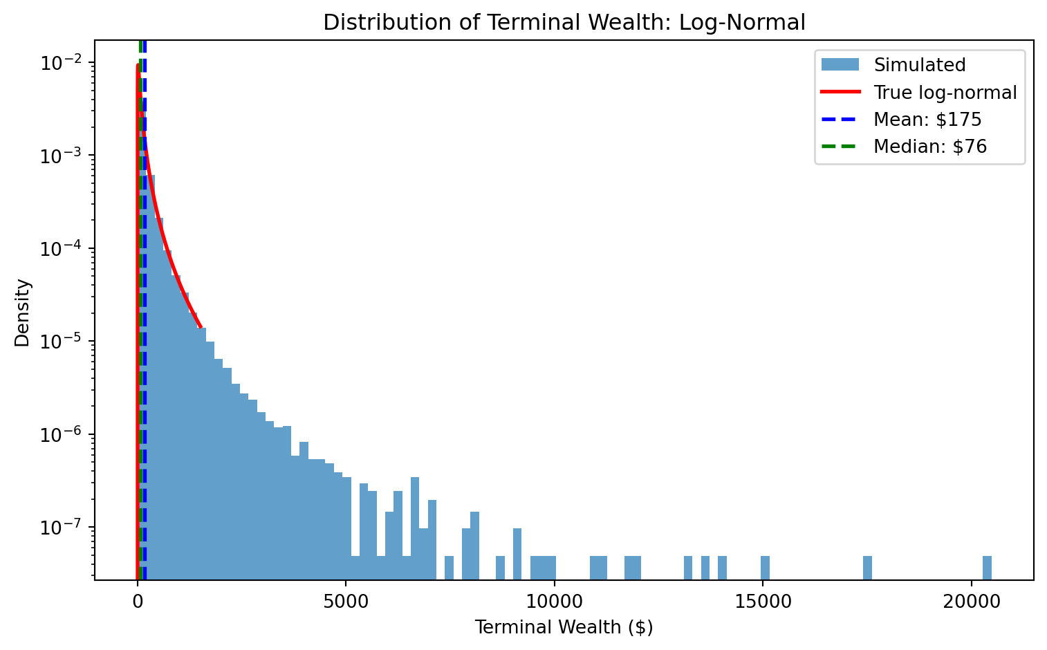
Over 60 years, starting with $1:
Median terminal wealth: $76
Mean terminal wealth: $177
The mean is 2.3× higher than the median
The mean is much higher than the median—the formulas tell us this must be true. But formulas can feel abstract. To really see what’s happening, we’ll run a Monte Carlo simulation.
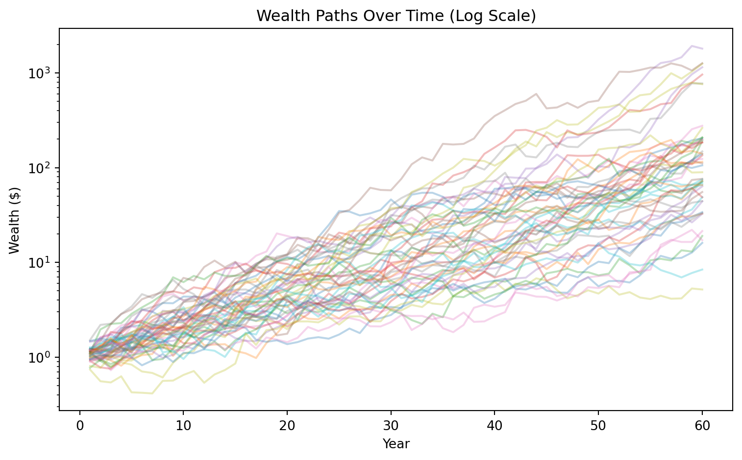
3.6 Simulating 100,000 Investors
The analytical results above tell us that if log returns are normal, wealth is log-normal, and the mean exceeds the median. But seeing this in action builds intuition that formulas alone can’t provide. We’re going to simulate 100,000 investors, each experiencing 60 years of independent random returns drawn from the same distribution. This is a numerical exercise meant to verify and illustrate the analytical work.
Here’s what we’ll do:
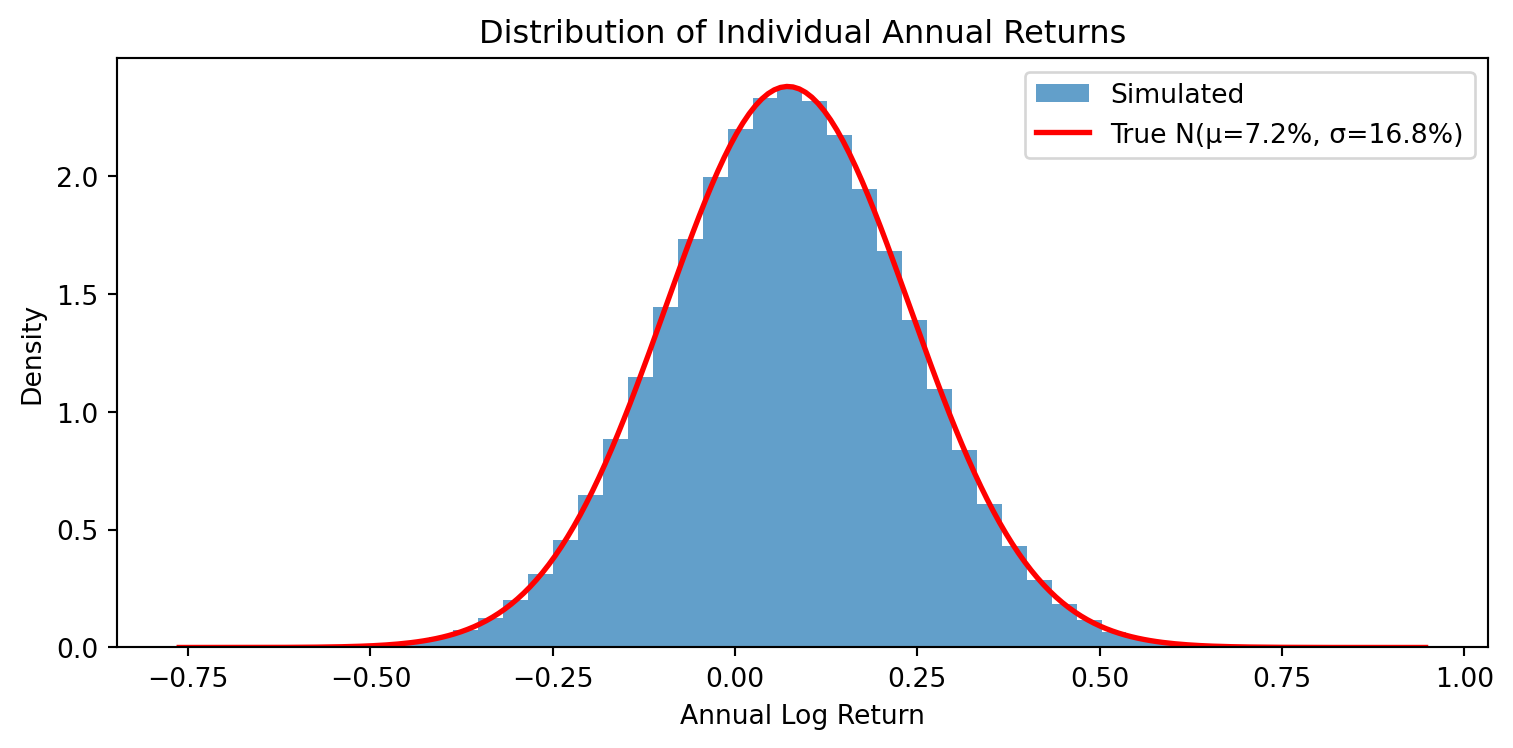
Generate returns: Draw 60 years of annual log returns for each of 100,000 investors from \(N(\mu, \sigma^2)\).
Watch the transformation: Follow how symmetric, normally distributed annual returns become asymmetric wealth through compounding.
Verify the formulas: Check that the simulated mean and median match our analytical predictions.
The key insight will be visual: we start with a symmetric bell curve (log returns), and through the simple act of exponentiating, we end up with a heavily right-skewed distribution (wealth) where most investors fall below the mean.
We draw 60 years of returns for each investor from \(N(\mu, \sigma^2)\):
np.random.seed(42)n_investors =100000# Each row = one investor, each column = one yearreturns = np.random.normal(mu, sigma, (n_investors, T))print(f"Shape: {returns.shape} (100,000 investors × {T} years)")
Most investors earn less than the expected value. The mean is not what a “typical” investor experiences—it’s inflated by the lucky few in the right tail.
4 Estimation Risk
4.1 From Known to Unknown Parameters
In the previous section, we treated \(\mu\) and \(\sigma^2\) as known parameters—as if we knew the true expected return and volatility with certainty. This is a useful theoretical exercise, but it’s not realistic. In practice, we must estimate these parameters from historical data. And estimation introduces its own source of uncertainty: estimation risk.
The distinction matters because we’ve already seen how uncertainty (in returns) inflates expected wealth through the variance boost. The same logic applies to uncertainty in our parameter estimates. If we’re uncertain about what \(\mu\) is, and we plug an estimate \(\hat{\mu}\) into an exponential formula, we’ll get another variance boost—on top of the one we already had.
The sample mean \(\hat{\mu} = \frac{1}{N}\sum_{i=1}^{N} r_i\) is an unbiased estimator of \(\mu\): on average across many samples, it equals the true mean. But the standard error\(SE(\hat{\mu}) = \sigma / \sqrt{N}\) tells us how much our estimate might deviate from truth in any given sample. Even with 100 years of annual data and 20% volatility, our estimate of \(\mu\) is only accurate to about \(\pm 2\%\). If the true \(\mu\) is around 8%, that’s a huge range of uncertainty—we might think it’s anywhere from 6% to 10%.
4.2 The Bias in Estimated Wealth
If we plug our estimate \(\hat{\mu}\) into the wealth formula, do we get an unbiased forecast?
Since \(\hat{\mu} \sim N(\mu, \sigma^2/N)\), the term \(T\hat{\mu}\) is also normal: \(T\hat{\mu} \sim N(T\mu, T^2\sigma^2/N)\). When we exponentiate, we apply the log-normal mean formula again: \[\mathbb{E}[\exp(T\hat{\mu})] = \exp\left(T\mu + \frac{T^2\sigma^2}{2N}\right)\]
The estimated wealth forecast \(\widehat{W}_T = W_0 \exp(T\hat{\mu} + T\sigma^2/2)\) has expected value: \[\mathbb{E}[\widehat{W}_T] = \mathbb{E}[W_T] \cdot \exp\left(\frac{T^2\sigma^2}{2N}\right)\]
The bias factor \(\exp(T^2\sigma^2/2N)\) is always greater than 1, so the estimated wealth systematically overestimates expected wealth. The same Jensen’s inequality logic applies: uncertainty in the estimate gets amplified through the exponential.
4.3 Correcting the Bias
To get an unbiased estimator of \(\mathbb{E}[W_T]\), we subtract the bias term from the exponent: \[\widehat{W}_T^{\text{unbiased}} = W_0 \cdot \exp\left(T\hat{\mu} + \frac{T\sigma^2}{2} - \frac{T^2\sigma^2}{2N}\right)\]
This adjustment is derived in Jacquier, Kane, and Marcus (2003), “Geometric or Arithmetic Mean: A Reconsideration,” Financial Analysts Journal.
4.4 Two Sources of Uncertainty
Our wealth forecast faces two distinct sources of uncertainty:
Return risk: Future returns are random. Variance contribution to log wealth: \(T\sigma^2\), growing linearly with horizon.
Estimation risk: We don’t know \(\mu\) exactly. Variance contribution to log wealth forecast: \(T^2\sigma^2/N\), growing with the square of horizon.
Estimation risk eventually dominates. For very long horizons, uncertainty about what \(\mu\)is matters more than the randomness of returns themselves.
4.5 Implications for Finance
This decomposition has profound implications for how we think about prediction and forecasting in finance.
Where is the randomness? It’s important to be precise about what’s random and what’s not. In Part I, returns \(r_t\) were random but we treated \(\mu\) as a known constant. That gave us the variance boost \(e^{T\sigma^2/2}\) from return risk alone. In Part II, we acknowledged that \(\mu\) is also uncertain—we only have an estimate \(\hat{\mu}\). Now our forecast \(\widehat{W}_T\) is a function of two random objects: the future returns (which we can’t observe yet) and our estimate of \(\mu\) (which varies across samples). Each source of randomness, when passed through the exponential function, creates its own variance boost.
Nonlinear transformations change distributions. In this chapter, the exponential function \(e^x\) was the culprit—it transformed normally distributed log returns into log-normally distributed wealth, creating variance boosts along the way. But this is a special case of a general principle that matters throughout machine learning.
ML often operates in nonlinear settings: neural networks apply nonlinear activation functions, tree-based methods partition space in complex ways, and many models transform inputs before making predictions. Whenever you pass a random variable through any nonlinear function, the output distribution differs from the input distribution—often in non-obvious ways. The mean of the output is not the function applied to the mean of the input (\(\mathbb{E}[f(X)] \neq f(\mathbb{E}[X])\)). Variance can expand or contract. Symmetric distributions can become skewed.
The lesson: you must understand the relationship between the distribution you’re modeling (here, log returns) and the distribution of what you ultimately care about (here, wealth). If there’s a nonlinear transformation in between, you can’t just plug in expected values and hope for the best.
Signal-to-noise and prediction: We’re trying to estimate the “signal” \(\mu\)—the true expected return—from data that’s overwhelmed by “noise” \(\sigma\). The standard error of our estimate is \(\sigma/\sqrt{N}\). With \(\sigma \approx 20\%\) and \(N = 100\) years, that’s a 2% standard error on a quantity that’s probably around 6-8%. The signal-to-noise ratio is terrible: we have roughly as much uncertainty about what \(\mu\)is as the magnitude of \(\mu\) itself. And this uncertainty, when compounded over long horizons and passed through the exponential, creates large biases.
The forecasting paradox: Here’s the uncomfortable implication. The further into the future we try to forecast, the less reliable our forecasts become—not just because more random returns accumulate (return risk grows as \(T\)), but because our uncertainty about parameters gets amplified more severely (estimation risk grows as \(T^2\)). Long-horizon forecasts look precise because they’re stated as single numbers, but they’re actually dominated by estimation uncertainty. A 30-year wealth projection depends more on whether you’ve estimated \(\mu\) correctly than on the actual sequence of returns.
This connects directly to why prediction is so hard in finance. We’re not just forecasting random returns; we’re also uncertain about the parameters that govern those returns. And both sources of uncertainty get amplified through the nonlinear transformation from returns to wealth.
5 Testing the Normality Assumption
5.1 Skewness and Kurtosis
Everything so far relied on the assumption that log returns are normally distributed. But assumptions should be tested, not just accepted. Is this one actually true?
The normal distribution has a very specific shape: perfectly symmetric, with thin tails that make extreme events exceedingly rare. Real data might differ in two key ways: it might be asymmetric (one tail longer than the other), or it might have fatter tails (extreme events more common than normal predicts). We measure these deviations with two statistics.
Skewness measures asymmetry: \[\gamma_1 = \frac{\mathbb{E}[(R - \mu)^3]}{\sigma^3}\] For a normal distribution, \(\gamma_1 = 0\). Negative skewness means the left tail is longer—large losses are more common than large gains. In finance, we often see slight negative skewness: crashes happen more often than equally-sized rallies.
Excess kurtosis measures tail heaviness relative to normal: \[\gamma_2 = \frac{\mathbb{E}[(R - \mu)^4]}{\sigma^4} - 3\] For a normal distribution, \(\gamma_2 = 0\). Positive kurtosis means “fat tails”—extreme events are more likely than normal predicts. The “-3” is there because a normal distribution has kurtosis of 3; we subtract this to get “excess” kurtosis relative to normal. A distribution with kurtosis of 25 has far more probability in its tails than normal.
5.2 Empirical Evidence
We can formally test normality using z-tests for skewness and kurtosis. Under the null hypothesis that returns are normally distributed, the sample skewness and kurtosis have known standard errors:
The z-statistics are \(z_{\text{skew}} = \hat{\gamma}_1 / \text{SE}(\hat{\gamma}_1)\) and \(z_{\text{kurt}} = \hat{\gamma}_2 / \text{SE}(\hat{\gamma}_2)\). Under normality, these are approximately standard normal, so we reject normality at the 5% level if \(|z| > 1.96\).
from scipy import stats# Compute daily log returnssp500['log_return'] = np.log(sp500['Close'] / sp500['Close'].shift(1))daily_returns = sp500['log_return'].dropna()# Summary statisticsskew = stats.skew(daily_returns)kurt = stats.kurtosis(daily_returns) # excess kurtosisprint(f"Data: {daily_returns.index.min().strftime('%Y-%m-%d')} to {daily_returns.index.max().strftime('%Y-%m-%d')}")print(f"Observations: {len(daily_returns):,} daily returns")print(f"\nSkewness: {skew:.3f} (normal = 0)")print(f"Excess kurtosis: {kurt:.1f} (normal = 0)")# Test statistics (under normality, these are approx standard normal)n_obs =len(daily_returns)z_skew = skew / np.sqrt(6/n_obs)z_kurt = kurt / np.sqrt(24/n_obs)print(f"\nTest statistics (reject normality if |z| > 1.96):")print(f" z_skewness = {z_skew:.1f}")print(f" z_kurtosis = {z_kurt:.1f}")
Both z-statistics are orders of magnitude larger than the critical value of 1.96. This is overwhelming statistical evidence against the normality assumption. The excess kurtosis z-statistic in the hundreds means the probability of observing this much kurtosis under normality is essentially zero.
# Standardize returnsdaily_mu = daily_returns.mean()daily_sigma = daily_returns.std()standardized = (daily_returns - daily_mu) / daily_sigmaprint("Extreme events (beyond k standard deviations):\n")print(f"{'k-sigma':<10}{'Actual':<10}{'Normal predicts':<18}{'Ratio':<10}")print("-"*50)for k in [3, 4, 5, 6]: actual = (abs(standardized) > k).sum() expected =len(daily_returns) *2* stats.norm.sf(k) ratio = actual / expected if expected >0else np.inf exp_str =f"{expected:.1f}"if expected >=0.1elsef"{expected:.1e}"print(f"{k}-sigma {actual:<10}{exp_str:<18}{ratio:,.0f}x")
Extreme events (beyond k standard deviations):

k-sigma    Actual     Normal predicts    Ratio
--------------------------------------------------
3-sigma    272        51.6               5x
4-sigma    107        1.2                88x
5-sigma    53         1.1e-02            4,837x
6-sigma    35         3.8e-05            928,055x
Four-sigma events happen roughly 90 times more often than normality predicts. The worst day in the sample—October 19, 1987 (Black Monday)—was a move of over 20 standard deviations, an event that should essentially never occur under normality.
5.3 Implications
The normality assumption is an approximation—a useful one, but an approximation nonetheless. It works reasonably well for “typical” days: the bell curve describes the middle of the return distribution fairly accurately. But it fails badly for extreme events, and extreme events are exactly what matter most for risk management.
Consider the practical implications:
Value at Risk (VaR): If you compute the 1% daily VaR assuming normality, you’re estimating the loss that should only be exceeded 1 day in 100. But if returns have fat tails, those catastrophic days happen more like 1 day in 50, or even 1 in 20. Your risk model would be dangerously overconfident.
Option pricing: The Black-Scholes model assumes log-normal prices (i.e., normal log returns). But real option prices reflect fat tails—out-of-the-money puts (insurance against crashes) are priced higher than Black-Scholes suggests, because traders know crashes happen more often than normal predicts.
Portfolio optimization: Mean-variance optimization (Markowitz) considers only the first two moments of returns. If returns have significant skewness or kurtosis, you’re ignoring information that matters to investors. Nobody wants a portfolio that maximizes expected return for a given variance if that portfolio is also prone to catastrophic left-tail events.
We continue using normal-based methods throughout this course because they’re tractable, widely used, and provide a foundation for more sophisticated approaches. But always remember: the tails are fatter than normal, and extreme events will happen more often than your models predict.
6 Why Prediction Is Hard
6.1 Autocorrelation
If yesterday’s return predicted today’s return, we could profit from it: buy after positive days, sell after negative days. This is called autocorrelation—the correlation of a time series with its own lagged values.
The empirical finding is sobering: autocorrelations in stock returns are tiny, typically \(|\rho| < 0.05\). With enough data, you can sometimes reject the null hypothesis that autocorrelation is zero (statistical significance), but the actual magnitude is so small that you can’t profit after transaction costs (economic significance). The market is remarkably efficient at eliminating simple patterns.
This shouldn’t be surprising. If yesterday’s return reliably predicted today’s, everyone would trade on it. Their trading would move prices until the pattern disappeared. Any easily exploitable pattern should be arbitraged away almost immediately.
6.2 In-Sample vs. Out-of-Sample
What about more sophisticated predictors? Researchers have tested hundreds of variables for predicting the equity premium: dividend yield, earnings-price ratio, interest rates, inflation, term spreads, default spreads, and many more. The sobering result, documented thoroughly by Goyal and Welch (2008) in “A Comprehensive Look at the Empirical Performance of Equity Premium Prediction” (Review of Financial Studies): most variables that predict returns in-sample fail to predict out-of-sample. The simple historical average is hard to beat.
6.3 The Signal-to-Noise Problem
Why is prediction so hard in finance? The fundamental issue is that financial returns have an extremely low signal-to-noise ratio. The “signal” is whatever true predictability exists—the part of next month’s return that can actually be forecast from today’s information. The “noise” is everything else: earnings surprises, geopolitical shocks, sentiment shifts, liquidity events, and countless other factors that move prices unpredictably.
In most applications of machine learning—image recognition, speech processing, recommendation systems—the signal-to-noise ratio is high. A photo of a cat contains overwhelming evidence that it’s a cat. But in finance, even if predictability exists, it’s tiny relative to the noise. Monthly stock returns have standard deviations around 4-5%, but the predictable component (if any) might be measured in basis points. You’re looking for a needle in a haystack, and the needle keeps moving.
This is why in-sample vs. out-of-sample evaluation matters so much more in finance than in other domains.
6.4 The IS/OOS Distinction
This distinction between in-sample and out-of-sample performance is arguably the central concern of machine learning:
In-sample (IS) refers to how well a model fits the data used to estimate it. You estimate coefficients using data from 1950-2000, then measure how well the model explains returns from 1950-2000.
Out-of-sample (OOS) refers to how well the model predicts new data it hasn’t seen. You estimate using 1950-2000, then measure how well it predicts returns from 2001-2020.
The problem is that in-sample performance is systematically overoptimistic. When you estimate a model, the coefficients adjust to fit everything in the sample—including the noise, the random fluctuations that won’t repeat. This is called overfitting. The model captures not just the true underlying patterns but also the specific idiosyncrasies of the estimation sample. Out-of-sample, those idiosyncrasies are different, so the fit degrades.
6.5 Preview: Setting Up a Return Prediction Regression
To make this concrete, let’s sketch how you would set up a simple return prediction exercise. Suppose you want to test whether the dividend yield predicts future stock market returns.
where \(r_{t+1}\) is next month’s market return and \(\text{DY}_t\) is this month’s dividend yield.
The IS/OOS split:
Estimation sample (IS): Use data from January 1950 to December 1999 to estimate \(\hat{\alpha}\) and \(\hat{\beta}\) using OLS.
Test sample (OOS): For each month from January 2000 onward, use the coefficients estimated from the past data to form a forecast: \(\hat{r}_{t+1} = \hat{\alpha} + \hat{\beta} \cdot \text{DY}_t\).
Evaluate: Compare the OOS forecasts to what actually happened. Did the model beat the simple historical average?
The key discipline: The coefficients used to make each OOS prediction must be estimated using only data available at the time of the forecast. You cannot use future information. This mimics what an investor could actually have done in real time.
We’ll implement this properly when we cover regression in Week 5, including how to measure forecast accuracy and test for statistical significance. For now, the takeaway is conceptual: any claim about predictability must be evaluated out-of-sample, using a proper time-series split that respects the flow of information.
6.6 Why Machine Learning?
This is why machine learning exists as a field. Much of this course is about techniques to avoid overfitting and improve out-of-sample performance:
Train/test splits: Never evaluate on data used for estimation
Cross-validation: Systematically rotate which data is held out
Regularization: Penalize model complexity to prevent overfitting
Ensemble methods: Average across many models to reduce variance
These techniques are responses to the fundamental challenge: with a low signal-to-noise ratio, it’s easy to find patterns that are noise, not signal. The only way to know the difference is to test on new data.
7 Summary
This chapter established the statistical framework we’ll use throughout the course. The key ideas are:
From Returns to Wealth: We work with log returns because they add over time, making them amenable to statistical analysis. But investors care about wealth, not log returns. The foundational assumption that log returns are normally distributed implies wealth is log-normally distributed. Expected wealth includes a variance boost: \(\mathbb{E}[W_T] = W_0 e^{T\mu + T\sigma^2/2}\). This boost arises from Jensen’s inequality—the convexity of the exponential function means that uncertainty inflates the mean. Since Mean \(>\) Median for log-normal distributions, most investors end up with less than the “expected” wealth. The expected value is a misleading summary statistic for wealth outcomes.
Estimation Risk: In practice, we don’t know \(\mu\)—we estimate it from historical data. This estimation uncertainty introduces another variance boost on top of the first one. The bias factor \(e^{T^2\sigma^2/2N}\) grows with the square of the time horizon, so estimation risk dominates for long-horizon forecasts. Any long-term wealth projection should be viewed with skepticism: it compounds two sources of upward bias.
The Normality Assumption Is Approximate: Testing the normality assumption against real S&P 500 data reveals significant deviations. Returns have excess kurtosis around 25, meaning fat tails. Extreme events—moves of 4 or more standard deviations—happen roughly 90 times more often than normal predicts. Black Monday (1987) was a 20+ sigma event, essentially impossible under normality. We use normal-based methods because they’re tractable, but we should never forget that tail risks are understated.
Prediction Is Hard: Financial returns have an extremely low signal-to-noise ratio—any predictable component is tiny relative to the noise. Autocorrelations are economically insignificant, and most variables that predict returns in-sample fail out-of-sample. The simple historical average is hard to beat. Proper evaluation requires splitting data into estimation (IS) and test (OOS) samples, using only past information to make each forecast. Overfitting—fitting noise rather than signal—is the central enemy. This is why machine learning matters: it provides tools to diagnose and combat overfitting.
These themes carry through the entire course. We’re always estimating something from noisy data, always at risk of overfitting, always needing to validate our models on data they haven’t seen. The techniques we’ll learn—cross-validation, regularization, ensemble methods—are all responses to these fundamental challenges.