Lecture 8: Ensemble Methods
RSM338: Machine Learning in Finance
1 Introduction
last lecture we introduced decision trees — a flexible, interpretable method that partitions the feature space using a sequence of yes/no questions. Trees can capture nonlinear relationships, handle mixed feature types without preprocessing, and produce decisions that a non-technical audience can follow from root to leaf. By almost any measure of convenience, trees are an ideal model.
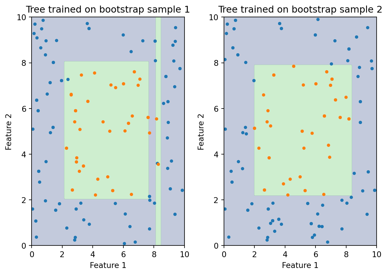
But we also saw their fatal flaw: high variance. Train a decision tree on one sample of loan applications and you might get a tree that splits first on credit score, then on DTI, then on income. Train another tree on a slightly different sample — say, swap out 10% of the observations — and the tree might split first on DTI, then on credit score, with completely different thresholds and a completely different structure. The predictions for the same borrower can change substantially depending on which training set the tree happened to see. This isn’t a subtle statistical concern — it means that the conclusions you draw from a single tree (which features matter, which borrowers are risky) are unreliable, because a different random draw of the data would have given you different conclusions.
The figure above illustrates the problem starkly. Both trees are trained on the same underlying data, but each sees a different bootstrap sample — a random draw with replacement from the original observations. The resulting decision boundaries look nothing alike. One tree might carve out a large region in the upper-right for one class; the other puts that same region in the opposite class. If you were making a business decision based on one of these trees, which one would you trust? Neither, really — and that’s the point. Any single tree is too unstable to rely on.
this lecture we fix the problem. The solution is to combine many trees into an ensemble — a committee of models whose collective prediction is far more stable and accurate than any individual member’s. We’ll study two families of ensemble methods. Random Forests take a parallel approach: train hundreds of trees independently, each on a slightly different version of the data, and average their predictions. Boosting takes a sequential approach: build trees one at a time, where each new tree specifically targets the mistakes that previous trees made. Both strategies produce dramatic improvements over single trees, and ensemble methods built on these ideas dominate applied machine learning on structured, tabular data — the kind of data that’s ubiquitous in finance.
2 The Ensemble Idea
2.1 Wisdom of Crowds
The ensemble idea has a surprisingly old pedigree. In 1906, the statistician Francis Galton attended a county fair where 800 people guessed the weight of an ox. Each individual guess was noisy — some too high, some too low, many wildly off. But when Galton computed the average of all 800 guesses, it was nearly perfect — closer to the true weight than almost any individual guess. The individual errors, being somewhat random and independent, cancelled each other out.
The same principle applies to statistical models. Suppose we train 100 different decision trees. Each tree has its own quirks and makes its own mistakes. Tree #17 might misclassify borrowers in one corner of the feature space; tree #42 might misclassify a different set of borrowers entirely. But if we average their predictions — or take a majority vote — the individual errors tend to cancel. The mistakes that are idiosyncratic to each tree wash out, and what remains is the signal that all the trees agree on. This is the ensemble principle: a committee of models outperforms any single member, not because each member is especially good, but because their mistakes are different enough to average away.
There’s a useful analogy to finance here. Diversification in a portfolio works for exactly the same reason. A single stock is volatile — its price depends on company-specific news, sector trends, and random noise. But a portfolio of 100 stocks is much less volatile, because the company-specific noise cancels out. The portfolio return converges toward the market return, which is the signal common to all stocks. Ensemble methods are doing the same thing with models instead of stocks: diversifying away the idiosyncratic “model-specific noise” to get a more stable prediction.
2.2 The Mathematics of Averaging
We can make this intuition precise. Suppose we have \(B\) models, each producing predictions with variance \(\sigma^2\). If the models are independent — their errors are completely uncorrelated — the variance of their average is:
\[\text{Var}\left(\frac{1}{B}\sum_{b=1}^{B} f_b(x)\right) = \frac{\sigma^2}{B}\]
With \(B = 100\) independent models, we cut the variance by a factor of 100. This is identical to the diversification formula from portfolio theory: the variance of an equally-weighted portfolio of \(B\) uncorrelated assets with equal variance \(\sigma^2\) is \(\sigma^2 / B\). Adding more models always reduces variance, and it does so rapidly at first (going from 1 to 10 models is a 10x reduction) before levelling off (going from 100 to 110 models barely matters).
But there’s a catch, and it’s the same catch that limits diversification in portfolios. The \(\sigma^2 / B\) formula assumes the models are independent — that their errors are completely uncorrelated. In practice, models trained on the same data are correlated. They tend to make similar mistakes, because they’re all responding to the same patterns (and the same noise) in the training data. If one tree overfits to a cluster of noisy observations in the upper-right corner of the feature space, other trees trained on the same data will likely do the same thing.
When models have pairwise correlation \(\rho\) (the Greek letter “rho,” measuring how similar the models’ prediction errors are), the variance of their average becomes:
\[\text{Var}\left(\bar{f}\right) = \rho\sigma^2 + \frac{1 - \rho}{B}\sigma^2\]
Look at this formula carefully. The second term, \((1 - \rho)\sigma^2 / B\), shrinks as we add more models — this is the part we can diversify away. But the first term, \(\rho\sigma^2\), doesn’t depend on \(B\) at all. No matter how many models we average, this term stays fixed. It’s the “systematic risk” of the ensemble, analogous to market risk in a portfolio. If \(\rho\) is close to 1 (models are nearly identical), then almost all the variance is in the first term and adding models barely helps. If \(\rho\) is close to 0 (models are nearly independent), then almost all the variance is in the second term and adding models helps enormously.
This formula tells us exactly what we need to do: make the models as different from each other as possible (reduce \(\rho\)) while keeping each one reasonably accurate (keep \(\sigma^2\) from exploding). The entire design of ensemble methods — bagging, random feature subsampling, boosting — is aimed at this tradeoff between individual model quality and inter-model diversity.
2.3 Three Strategies for Diversity
How can we train models on the same dataset but get them to disagree? There are three main strategies, and each gives rise to a different ensemble method:
| Strategy | How it works | Method |
|---|---|---|
| Different data | Train each model on a random subset of observations | Bagging |
| Different features | At each split, only consider a random subset of features | Random Forests |
| Sequential correction | Each new model focuses on the mistakes of previous ones | Boosting |
The first two strategies — different data and different features — are both forms of randomization. We inject randomness into the training process so that each tree sees a slightly different version of the problem. The trees end up learning slightly different patterns, which makes them less correlated with each other. These are “parallel” strategies: the trees are independent of each other and can be trained simultaneously.
The third strategy — sequential correction — is fundamentally different. Instead of making trees independent, it makes them complementary. Each tree is designed to fix the specific mistakes made by the trees that came before it. The trees are highly dependent on each other (each one is built to compensate for the others), but the ensemble improves incrementally with each addition. This is a “sequential” strategy: tree \(m\) can only be built after trees \(1\) through \(m-1\) are complete.
2.4 Bootstrap Sampling
Before we can talk about bagging, we need to understand the sampling mechanism it relies on. Bootstrap sampling means drawing \(n\) observations from the training data with replacement. “With replacement” means that after we draw an observation, we put it back in the pool before drawing the next one. The result is that some observations get picked multiple times, while others are left out entirely.
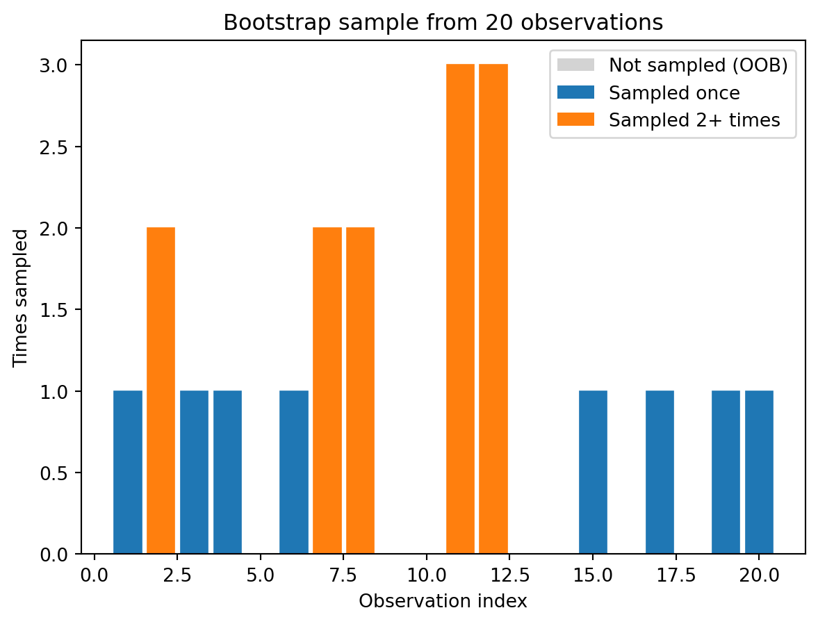
Unique observations in this bootstrap sample: 13 out of 20 (65%)This might seem like a strange thing to do — why would we want duplicates in our training data and gaps where some observations are missing? The answer is that it creates variation. Each bootstrap sample is a slightly different version of the original dataset, and a model trained on one bootstrap sample will differ from a model trained on another. That’s exactly the diversity we need.
A useful fact: on average, each bootstrap sample contains about 63.2% of the unique observations. The math behind this is worth knowing. For any single observation, the probability of not being selected in one draw is \((n-1)/n\). Across \(n\) independent draws, the probability of never being selected is \(((n-1)/n)^n\), which converges to \(1/e \approx 0.368\) as \(n\) grows. So about 36.8% of observations are left out of any given bootstrap sample. These left-out observations are called out-of-bag (OOB) observations, and they’ll turn out to be very useful for model validation — essentially giving us a free test set for each tree.
2.5 Bagging: Bootstrap Aggregation
Bagging (short for “bootstrap aggregation,” introduced by Breiman in 1996) is the simplest ensemble method. It combines bootstrap sampling with model averaging:
- Draw \(B\) bootstrap samples from the training data
- Train one decision tree on each bootstrap sample
- To predict a new observation: have all \(B\) trees vote (classification) or average their predictions (regression)
\[\hat{y}(x) = \text{majority vote of } \{\hat{f}_1(x), \hat{f}_2(x), \ldots, \hat{f}_B(x)\}\]
Each tree sees a slightly different version of the data, so they learn slightly different patterns. The trees that overfit to noise in one direction are cancelled out by trees that overfit in another direction, and the ensemble vote smooths out the individual quirks. In classification, if 70 out of 100 trees predict “default” for a given borrower, the ensemble predicts “default” — and that prediction is far more reliable than any single tree’s verdict.
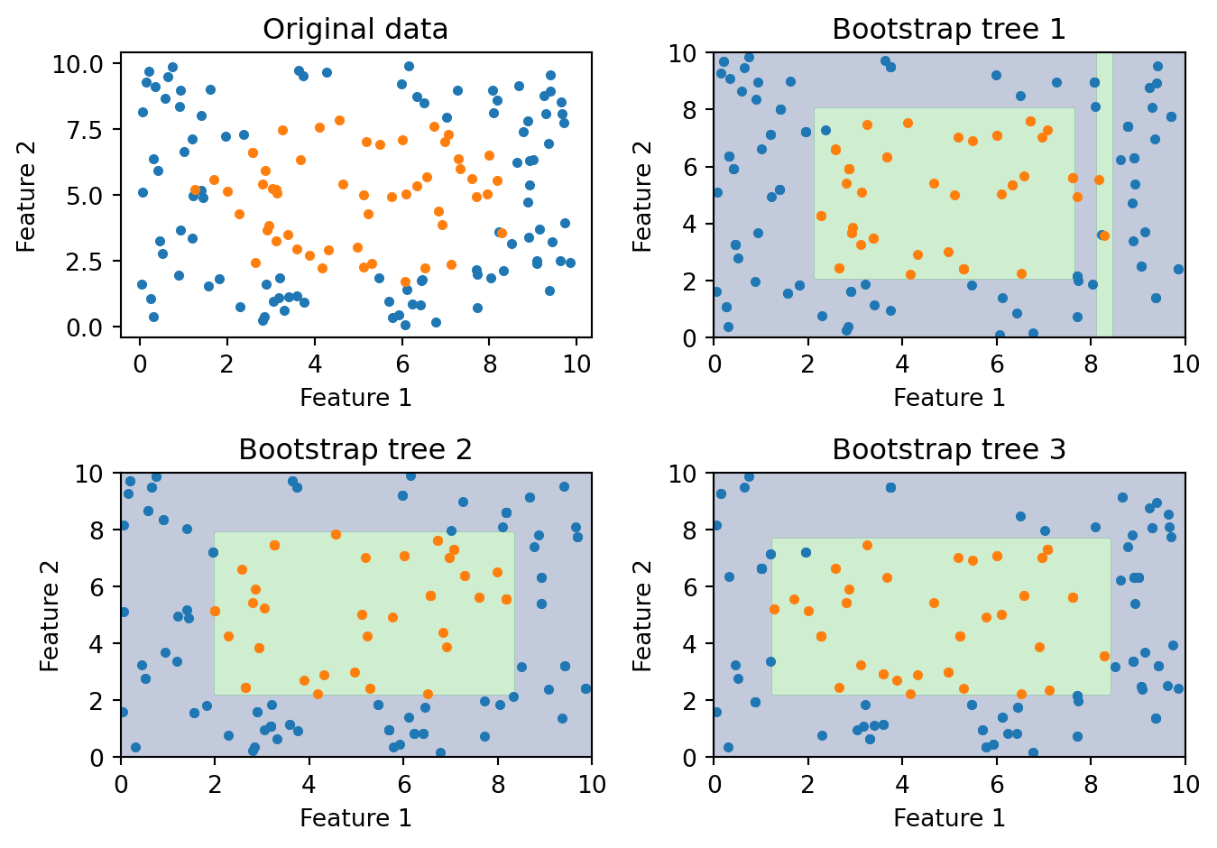
The figure shows three trees, each trained on a different bootstrap sample from the same underlying data. Each tree learns a somewhat different decision boundary. The differences come from two sources: the bootstrap samples contain different observations (some points are in, some are out, some appear twice), and the trees’ greedy splitting algorithm amplifies those differences (a slightly different dataset can change the root split, which changes everything downstream). When we combine all three — or better yet, hundreds of trees — the idiosyncratic boundaries average out and the ensemble captures the true underlying pattern more reliably than any individual tree.
Bagging is a clear improvement over single trees, but it has a limitation. If one feature is much stronger than the rest, every bagged tree will split on it first. Think about credit scoring: if FICO score is by far the best predictor of loan default, then every bootstrap sample still contains FICO as a feature, and the greedy splitting algorithm will put FICO at the root of every tree. The trees end up looking very similar — same first split, similar second split, and so on. They’re all correlated because they’re all dominated by the same strong feature. Going back to our variance formula, \(\rho\) remains high, and the variance reduction from averaging is limited. In portfolio terms, it’s like “diversifying” by buying 100 stocks that are all in the same sector. We need a way to force the trees apart.
3 Random Forests
3.1 The Algorithm
Random Forests (Breiman, 2001) solve bagging’s correlation problem with one additional twist: at each split in each tree, only a random subset of features is considered as candidates. The full algorithm is:
- Draw a bootstrap sample from the training data
- Grow a tree, but at each split:
- Randomly select \(m_{\text{try}}\) features out of the \(p\) available
- Find the best split among only those \(m_{\text{try}}\) features
- Repeat steps 1–2 for \(B\) trees
- Predict by majority vote (classification) or average (regression)
The feature subsampling happens at every split, not just once per tree. So even within a single tree, different nodes see different subsets of features. This injects randomness at a very granular level, ensuring that even two trees trained on the same bootstrap sample will end up with different structures because they considered different features at each decision point.
Notice that Random Forests combine both sources of randomness: different observations (via bootstrap sampling) and different features (via random subsampling at each split). The bootstrap sampling gives each tree a slightly different dataset; the feature subsampling prevents all trees from being dominated by the same strong features. Together, these two mechanisms push the pairwise correlation \(\rho\) down, making the averaging in the ensemble much more effective.
3.2 How Many Features Per Split?
The parameter \(m_{\text{try}}\) (sometimes written max_features in scikit-learn) controls how many features each split is allowed to see. This is the key tuning knob that governs the diversity-accuracy tradeoff. Common defaults are:
| Task | Default \(m_{\text{try}}\) | With \(p = 16\) features |
|---|---|---|
| Classification | \(\sqrt{p}\) | 4 features per split |
| Regression | \(p/3\) | ~5 features per split |
These defaults come from empirical experience across many datasets and work well in most situations. To understand why, think about the extremes. With \(m_{\text{try}} = 1\), each split is forced to use a single randomly chosen feature, regardless of whether it’s informative. The trees are maximally diverse (very low \(\rho\)) but individually terrible — many splits are on irrelevant features, so each tree has high bias and low accuracy. With \(m_{\text{try}} = p\), every feature is available at every split, and the algorithm reduces to ordinary bagging. Each tree is individually as good as possible, but they’re all similar (high \(\rho\)), limiting the benefit of averaging. The defaults of \(\sqrt{p}\) (classification) and \(p/3\) (regression) hit a sweet spot: enough features per split that each tree is a reasonable model, but few enough that the trees differ substantially from each other.
3.3 Why Feature Subsampling Helps
To make this concrete, imagine you have 10 features for predicting loan default, but FICO score is the strongest predictor by a wide margin. Without feature subsampling (i.e., plain bagging with \(m_{\text{try}} = p\)), the greedy algorithm will put FICO at the root of every single tree, because no other feature can beat it in terms of information gain. The top of every tree looks the same, and the lower splits are only slightly different. The trees are highly correlated, and we’re not getting much benefit from averaging 500 versions of essentially the same model.
Now suppose we use \(m_{\text{try}} = 3\). At each split, the algorithm randomly selects 3 of the 10 features and picks the best among those 3. At the root of tree #1, maybe the random draw includes FICO, DTI, and home ownership — FICO wins. But at the root of tree #2, the random draw might include income, employment length, and loan amount — no FICO this time. Tree #2 is forced to start with income or employment length, and its entire structure develops differently as a result. It discovers patterns in the data that FICO-dominated trees would never find. Maybe high income combined with high DTI is a risk signal that only becomes visible when FICO isn’t hogging all the attention.
Each individual tree is slightly less accurate than it would be with access to all features — sometimes the best available feature is #3 out of 10 rather than #1. But the ensemble is substantially better because the trees are much less correlated. The errors that tree #1 makes (because it’s FICO-dominated) are different from the errors that tree #2 makes (because it’s income-dominated), and they cancel out when averaged. The whole is greater than the sum of its parts.
3.4 Out-of-Bag Error Estimation
One of the most useful properties of Random Forests is that they come with a built-in validation mechanism — no separate test set or cross-validation loop required. Recall that each bootstrap sample leaves out about 36.8% of the training observations. For any given observation \(i\), roughly a third of the trees in the forest never saw it during training. We can collect predictions for observation \(i\) from only those trees, and compare to the true label. Doing this for every observation gives us the out-of-bag (OOB) error estimate.
The procedure is:
- For each training observation \(i\), identify all trees where \(i\) was out-of-bag (i.e., not in that tree’s bootstrap sample)
- Collect predictions from those trees only and take a majority vote (or average for regression)
- Compare the OOB prediction to the true label
- Average the error across all observations
The OOB error is approximately equivalent to leave-one-out cross-validation, but it comes for free — it’s a natural byproduct of the bootstrap sampling process. This is a real practical advantage. Cross-validation requires refitting the model multiple times (e.g., 5 or 10 times for 5-fold or 10-fold CV), which can be expensive for large datasets. OOB error requires fitting the forest only once and gives a comparably reliable estimate of out-of-sample performance. When you see the oob_score=True parameter in scikit-learn’s RandomForestClassifier, this is what it computes.
3.5 Feature Importance
Random Forests provide a natural way to measure which features matter most for prediction. Since the forest contains hundreds of trees, each making hundreds of splits, we can aggregate information across all of these to get stable importance rankings.
Impurity-based importance (the default in scikit-learn) works by looking at every split in every tree and measuring how much it reduced impurity (Gini or entropy). For each feature, we sum up the total impurity reduction across all splits in all trees that used that feature. Features that appear in many splits and produce large drops in impurity — especially near the top of the trees, where there are more observations to split — get ranked as more important. A feature that the forest never splits on (or splits on only rarely, and with small impurity reductions) gets a low importance score.
Permutation importance takes a different approach: randomly shuffle one feature’s values and measure how much the model’s accuracy drops. The logic is simple — if a feature is genuinely useful for prediction, then scrambling its values should hurt the model’s accuracy. If a feature is irrelevant, scrambling it changes nothing. To compute permutation importance, we take the trained forest, evaluate it on a test set to get a baseline accuracy, then for each feature: shuffle that feature’s column, re-evaluate accuracy, and record the drop. The size of the accuracy drop is the feature’s importance.
Permutation importance is generally considered more reliable than impurity-based importance, particularly when features are correlated or when some features have many more unique values than others (impurity-based importance can be biased toward high-cardinality features). But impurity-based importance is faster to compute and often gives similar rankings.
3.6 Random Forests in Python
from sklearn.ensemble import RandomForestClassifier
from sklearn.datasets import make_classification

# Generate synthetic data
X_synth, y_synth = make_classification(
    n_samples=500, n_features=10, n_informative=5,
    random_state=42
)

# Train a Random Forest
rf = RandomForestClassifier(
    n_estimators=100,      # number of trees
    max_features='sqrt',   # features per split = sqrt(p)
    oob_score=True,        # compute out-of-bag accuracy
    random_state=42
)
rf.fit(X_synth, y_synth)

print(f"OOB accuracy: {rf.oob_score_:.3f}")
print(f"Training accuracy: {rf.score(X_synth, y_synth):.3f}")
OOB accuracy: 0.906
Training accuracy: 1.000The gap between training accuracy and OOB accuracy tells us something about overfitting. Training accuracy is measured on the same data the forest was trained on, so it’s optimistically biased. OOB accuracy is measured on held-out observations for each tree, so it’s a more honest estimate of how the model would perform on genuinely new data. If the gap is large, the model is overfitting; if the gap is small, the model generalizes well. For Random Forests, the gap is typically modest because the averaging across many trees regularizes the model naturally.
3.7 How Many Trees?
A natural question is: how many trees do we need? The answer, from both theory and practice, is reassuring: more trees never hurts. Unlike most models, where increasing complexity eventually leads to overfitting, Random Forests only get more stable (or stay the same) as we add more trees. Each additional tree contributes one more independent opinion to the vote, and the law of large numbers ensures that the ensemble prediction converges.
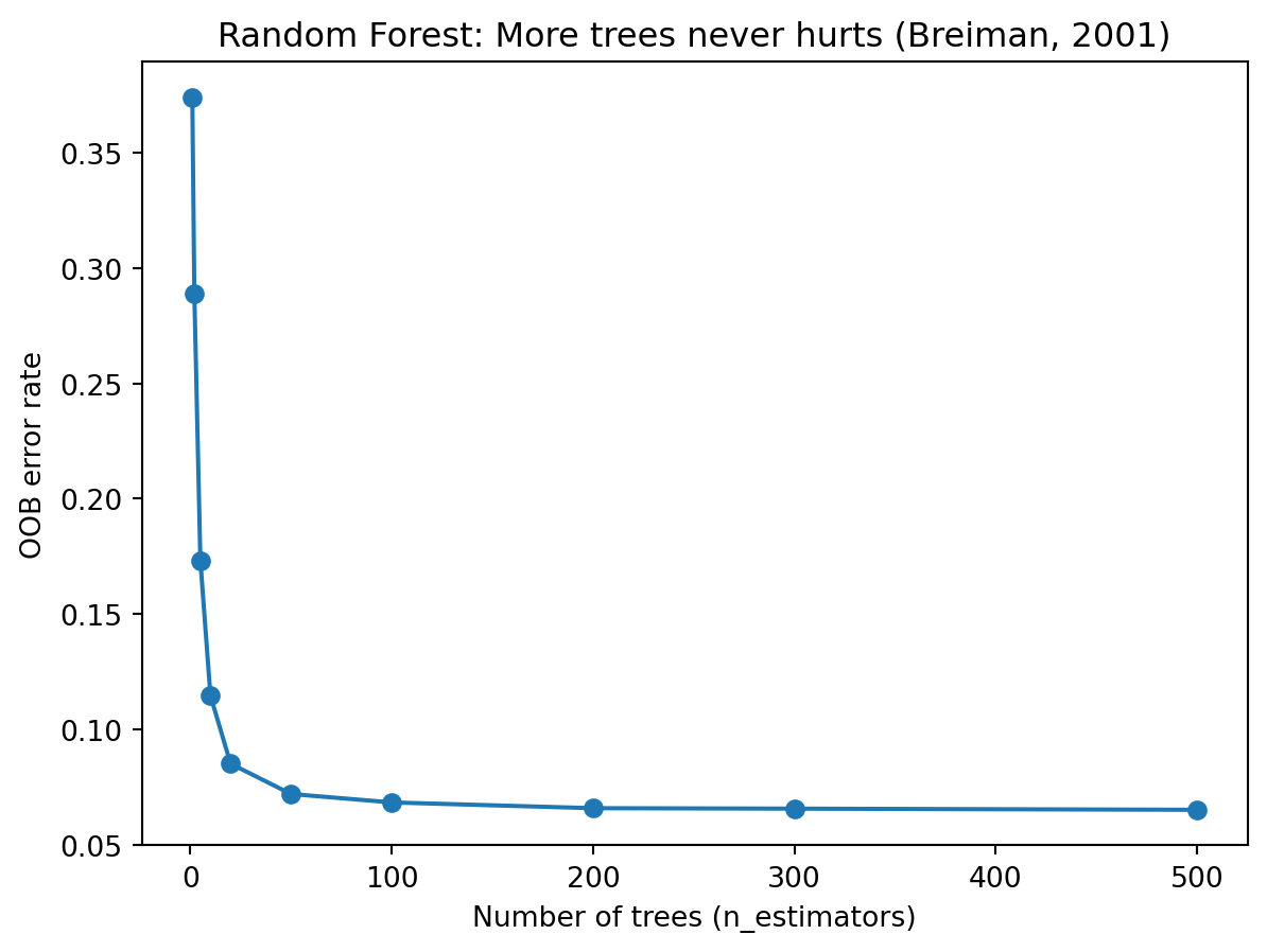
The plot shows OOB error dropping sharply as we go from 1 to about 50 trees, then levelling off. Beyond 100 or 200 trees, the improvement is negligible — the ensemble has already converged. The only cost of adding more trees is computation time. In practice, 100–500 trees is a common range. If you can afford the computation, there’s no reason not to use more, but you get diminishing returns after the error curve flattens out.
This “more is always better (or at least neutral)” property is specific to Random Forests and does not hold for boosting methods, where too many rounds can lead to overfitting. It comes from the fact that each tree in a Random Forest is trained independently. Adding tree #501 doesn’t change trees #1 through #500 — it just adds one more vote. The ensemble can only become more stable, never less stable. Breiman (2001) proved this convergence result formally.
3.8 Visualizing Variance Reduction
To see the variance-reduction effect as concretely as possible, consider a regression example. We generate noisy data from a sine curve and fit both a single tree and a Random Forest.
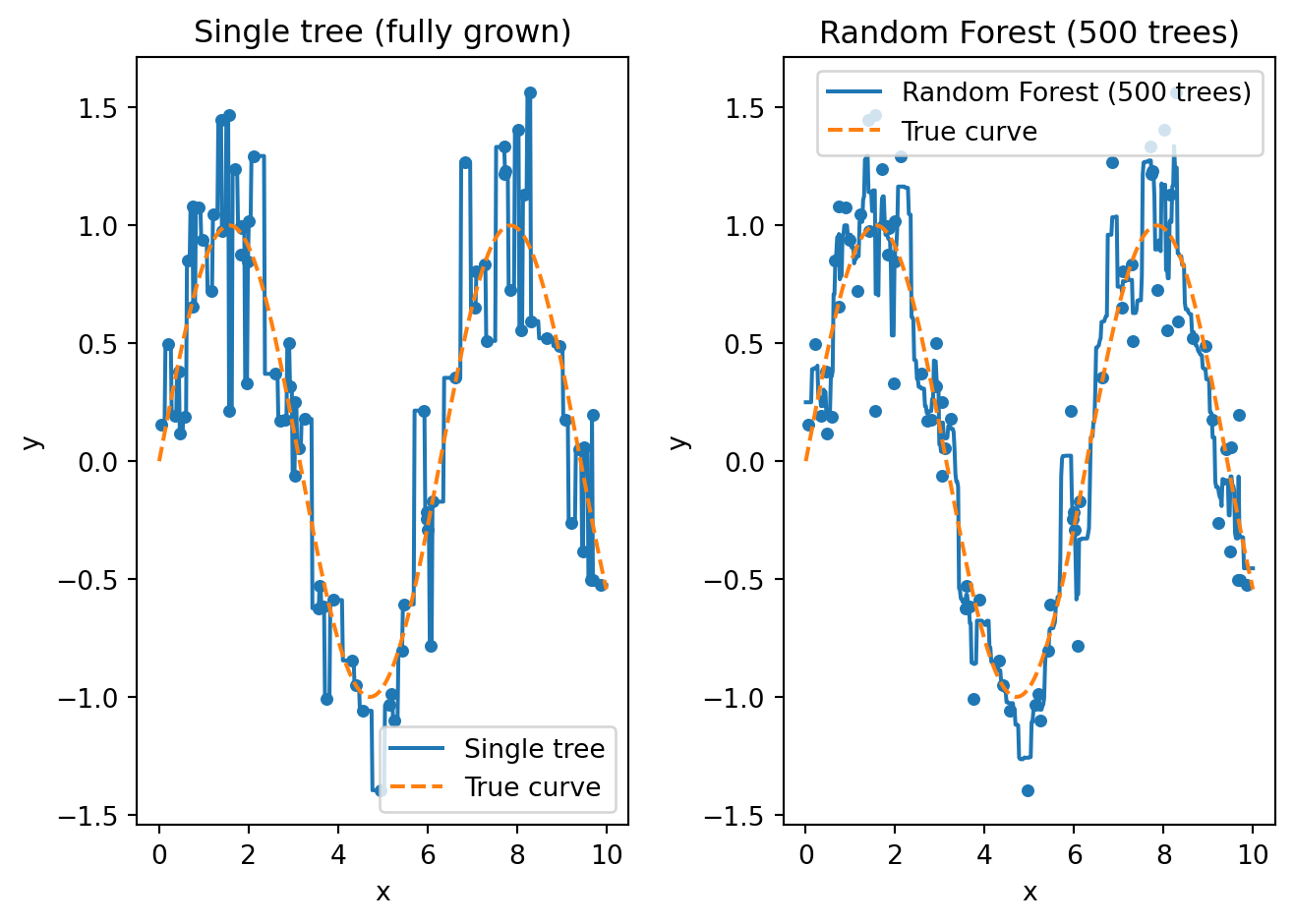
The left panel shows a single fully-grown tree. It memorizes every training point, producing a jagged step function that jumps up and down to hit each observation exactly. This is pure overfitting — the tree treats every bit of noise as if it were signal, resulting in predictions that would be wildly wrong for new observations between the training points.
The right panel shows what happens when we average 500 such trees. Each tree individually is just as jagged and overfit as the one on the left. But because each tree was trained on a different bootstrap sample and considered different random features at each split, the 500 trees overfit in different ways. Tree #1 might spike upward at \(x = 3.2\) because of a noisy training point; tree #2 might spike downward at the same location because it saw different points. When we average all 500 trees, these spikes cancel out and the result is a smooth curve that closely tracks the true sine function. This is variance reduction in action: each individual tree has high variance, but their average has low variance.
3.9 Hyperparameters
Random Forests have several hyperparameters, but they’re unusual among machine learning models in that the defaults work well for most problems. Here are the main ones:
| Parameter | What it controls | Typical range |
|---|---|---|
n_estimators |
Number of trees in the forest | 100–1000 (more is better, but slower) |
max_features |
Features considered per split | 'sqrt' (classification), p/3 (regression) |
max_depth |
Maximum depth of each tree | None (fully grown) or 10–30 |
min_samples_leaf |
Minimum observations in a leaf | 1–10 |
The most important decision is n_estimators — use as many trees as your computational budget allows. After that, max_features is the main tuning parameter, though the defaults (\(\sqrt{p}\) for classification, \(p/3\) for regression) are hard to beat. You might consider limiting max_depth or increasing min_samples_leaf if you’re concerned about overfitting, but in practice the averaging across many trees already provides strong regularization, so these constraints are less necessary than they are for single trees.
This robustness to hyperparameter choices is a major practical advantage of Random Forests. With many other models (ridge regression, lasso, k-NN, neural networks), performance is highly sensitive to the hyperparameter settings, and cross-validation is essential. With Random Forests, you can often use the defaults and get a competitive model without any tuning at all.
4 Boosting
4.1 A Different Philosophy
Random Forests reduce error by averaging many independent, strong models. Each tree is grown deep (high accuracy, high variance), and the averaging reduces the variance. Boosting takes the opposite approach: start with weak models and gradually build them into a strong one by correcting errors sequentially.
Think of it like preparing for a difficult exam. A Random Forest approach would be: take 100 practice exams under slightly different conditions, average your answers. A boosting approach would be: take one practice exam, identify the questions you got wrong, study those topics intensively, take another practice exam, identify remaining weaknesses, study those, and so on. Each round of study is modest (you’re not trying to learn everything at once), but each round targets the specific gaps left by previous rounds. After many rounds, you’ve addressed every weakness.
Boosting does the same thing with models. Each new tree is a “weak learner” — deliberately small, shallow, and limited. It doesn’t try to solve the whole prediction problem. Instead, it focuses on the specific observations that the current ensemble still gets wrong. After many rounds of these targeted corrections, the ensemble has addressed errors across the entire dataset.
4.2 Weak Learners
The building blocks of boosting are weak learners — models that are only slightly better than random guessing. For binary classification, “slightly better than random” means accuracy above 50%. The typical weak learner is a decision stump: a tree with just one split (depth = 1). A stump can only ask one question (“Is FICO > 700?”), so it’s a very crude model on its own. It captures one feature’s effect on the outcome and ignores everything else.
This seems like a terrible starting point. How can a model that’s barely better than a coin flip be useful? Schapire (1990) proved a remarkable theoretical result that answers this question: any collection of weak learners can be combined into a strong learner with arbitrarily high accuracy, as long as each weak learner is slightly better than random. You don’t need individual models to be good — you just need each one to contribute a small amount of information that the others haven’t already captured. Over many rounds, these small contributions accumulate into an ensemble that can match or exceed the performance of much more complex individual models.
In practice, gradient boosting typically uses small trees of depth 3–6 rather than stumps, because a depth-3 tree can capture some interaction effects (the effect of feature A depends on feature B) that a stump cannot. But the principle is the same: each tree is deliberately small and weak, and the boosting process builds accuracy incrementally.
4.3 AdaBoost: The Original Boosting Algorithm
AdaBoost (Adaptive Boosting, Freund & Schapire, 1997) was the first practical boosting algorithm, and understanding it helps build intuition for the more general gradient boosting framework that followed.
The core idea is to maintain a set of weights over the training observations, one weight per observation, that control how much each observation matters. Initially all weights are equal: \(w_i = 1/n\). In each round, we train a weak learner on the weighted data, evaluate how well it does, and then increase the weights on the misclassified observations so the next round’s learner will pay more attention to them. Observations that are easy to classify correctly get their weights reduced; observations that are hard to classify get their weights boosted. Over many rounds, the algorithm pours more and more effort into the difficult cases.
More formally, in each round \(m = 1, 2, \ldots, M\):
- Fit a weak learner \(h_m(x)\) on the weighted training data
- Compute the weighted error — the total weight on misclassified points: \[\varepsilon_m = \frac{\sum_{i:\, h_m(x_i) \neq y_i} w_i}{\sum_{i=1}^{n} w_i}\]
- Compute this learner’s vote weight (Greek letter “alpha”): \[\alpha_m = \frac{1}{2}\ln\!\left(\frac{1 - \varepsilon_m}{\varepsilon_m}\right)\]
- Update weights — multiply each misclassified observation’s weight by \(e^{\alpha_m}\) and each correctly classified observation’s weight by \(e^{-\alpha_m}\), then renormalize so weights sum to 1
The vote weight formula \(\alpha_m\) deserves some attention. When a learner makes few mistakes (\(\varepsilon_m\) close to 0), the fraction \((1 - \varepsilon_m)/\varepsilon_m\) is large, so \(\alpha_m\) is large — this learner gets a loud voice in the final vote. When a learner does poorly (\(\varepsilon_m\) close to 0.5, barely better than random), the fraction approaches 1, so \(\alpha_m\) is near 0 — this learner’s vote barely counts. If a learner is worse than random (\(\varepsilon_m > 0.5\)), \(\alpha_m\) becomes negative, which effectively flips its predictions. The formula automatically calibrates how much to trust each learner based on its accuracy.
The final prediction is a weighted vote across all \(M\) learners:
\[\hat{y}(x) = \text{sign}\!\left(\sum_{m=1}^{M} \alpha_m \, h_m(x)\right)\]
AdaBoost is formulated for binary classification where the class labels are coded as \(y_i \in \{-1, +1\}\) (not 0 and 1, as in logistic regression). Each stump \(h_m(x)\) also outputs \(-1\) or \(+1\), so the weighted sum \(\sum \alpha_m h_m(x)\) is a real number whose sign tells us the predicted class: positive means predict \(+1\), negative means predict \(-1\). The magnitude tells us the ensemble’s confidence — a sum far from zero means the trees agree strongly, while a sum near zero means the vote was close.
4.4 Comparing the Two Ensemble Strategies
At this point it’s worth stepping back and comparing the two ensemble strategies we’ve seen, because they represent fundamentally different philosophies for combining models:
| Bagging / Random Forest | Boosting | |
|---|---|---|
| Training | Parallel (trees are independent) | Sequential (each tree depends on previous) |
| Tree type | Full-sized, deep trees | Shallow trees (weak learners) |
| Primary benefit | Reduces variance | Reduces bias (and variance) |
| Overfitting risk | Low (more trees never hurts) | Higher (can overfit if too many rounds) |
| Sensitivity to noise | Robust | More sensitive |
| Computation | Easy to parallelize | Harder to parallelize |
The distinction between “reduces variance” and “reduces bias” is worth unpacking. A single deep tree has low bias (it can fit complex patterns) but high variance (it’s unstable). Random Forests keep the low bias of deep trees and reduce the variance through averaging. A single shallow tree has high bias (it’s too simple to capture complex patterns) but low variance (it’s stable). Boosting reduces the bias by combining many shallow trees, each of which corrects a different part of the error. The two approaches are attacking different parts of the bias-variance tradeoff, which is why they’re both useful and why the best choice depends on the data.
The overfitting distinction is also practically important. With Random Forests, you can always safely add more trees — the error will decrease or plateau, never increase. With boosting, too many rounds can cause the model to overfit, particularly if the learning rate is high. This means boosting requires more careful tuning: you need to choose the number of rounds, the learning rate, and the tree depth in a way that balances accuracy against overfitting, typically using cross-validation.
4.5 From AdaBoost to Gradient Boosting
AdaBoost works by re-weighting observations — misclassified points get higher weights. Gradient Boosting (Friedman, 2001) generalized this idea in a way that’s both more flexible and more powerful: instead of adjusting observation weights, fit each new tree directly to the residuals (errors) of the current model. If the ensemble currently predicts \(\hat{y}_i = 3.2\) for observation \(i\) but the true value is \(y_i = 5.0\), the residual is \(5.0 - 3.2 = 1.8\). The next tree is trained to predict these residuals — in other words, to predict what the current model is getting wrong. Add that tree’s predictions to the ensemble, and the residuals shrink. Repeat.
The name “gradient boosting” comes from a connection to gradient descent, the optimization algorithm we studied in Lecture 5. Recall that gradient descent updates parameters by taking a step in the direction that reduces the loss function:
\[\theta_{t+1} = \theta_t - \eta \, \nabla L(\theta_t)\]
where \(\eta\) (Greek letter “eta”) is the learning rate and \(\nabla L\) is the gradient of the loss function. Gradient boosting applies this same idea, but instead of updating numerical parameters \(\theta\), we update the model’s prediction function by adding a new tree. Let \(F_m(x)\) be the ensemble’s prediction after \(m\) rounds — the running total of every tree’s contribution so far. And let \(h_m(x)\) be the new tree fit in round \(m\) — the next correction. The update rule is:
\[F_m(x) = F_{m-1}(x) + \eta \cdot h_m(x)\]
Each round takes yesterday’s prediction and nudges it in the direction that reduces the loss. The learning rate \(\eta\) controls how big the nudge is. And the direction of the nudge is determined by fitting a tree to the negative gradient of the loss, which for squared-error loss is exactly the residual \(y_i - F_{m-1}(x_i)\).
The advantage of this gradient-based formulation over AdaBoost’s re-weighting is generality. AdaBoost is specifically designed for classification with 0/1 error. Gradient boosting works with any differentiable loss function — squared error for regression, log-loss for classification, quantile loss for prediction intervals, and so on. You just swap in a different loss function and the algorithm automatically fits trees to the appropriate residuals. This flexibility is why gradient boosting has largely superseded AdaBoost in practice.
5 Gradient Boosting and XGBoost
5.1 The Full Algorithm
Here is the gradient boosting algorithm in detail. Given training data, a loss function \(L\), number of rounds \(M\), and learning rate \(\eta\):
Start with a constant prediction: \(F_0(x) = \arg\min_c \sum_{i=1}^n L(y_i, c)\)
This is just the best constant guess — for squared-error loss, it’s the mean of the training labels; for log-loss, it’s the log-odds of the positive class.
For \(m = 1, 2, \ldots, M\):
Compute pseudo-residuals for each observation — how far off the current model is, measured in the direction of steepest descent: \[r_{im} = -\frac{\partial L(y_i, F_{m-1}(x_i))}{\partial F_{m-1}(x_i)}\]
Fit a small tree \(h_m\) to the pseudo-residuals \(\{(x_i, r_{im})\}\)
Update the model: \[F_m(x) = F_{m-1}(x) + \eta \cdot h_m(x)\]
The term “pseudo-residuals” is used because, for loss functions other than squared error, they aren’t literally the residuals \(y_i - F_{m-1}(x_i)\). They’re the negative gradient of the loss with respect to the prediction, which generalizes the notion of “how wrong are we” to arbitrary loss functions. For squared-error loss, the negative gradient works out to exactly \(y_i - F_{m-1}(x_i)\), so the pseudo-residuals are the ordinary residuals. Each new tree literally predicts what the current model is getting wrong.
When the pseudo-residuals hit zero everywhere, the negative gradient of the loss is zero — the same condition as being at a minimum in ordinary calculus. There is no direction to move that would reduce the loss further, and the algorithm has converged. In practice, we stop after \(M\) rounds (before reaching convergence) as a form of regularization, because running to full convergence would overfit.
5.2 Why Shallow Trees?
This is one of the most common sources of confusion when students first learn about ensemble methods. In Random Forests, each tree is grown deep — as deep as possible, with no pruning. The individual trees need to be accurate on their own because we’re just averaging them. In gradient boosting, the strategy is reversed: each tree should be deliberately shallow, typically depth 3 to 6.
Why? Because each tree in gradient boosting isn’t trying to solve the whole problem. It’s making a small, targeted correction to the current ensemble. If tree #50 is correcting the errors left over from trees #1 through #49, there shouldn’t be much left to correct — the residuals are small and the corrections should be small too. A deep tree would overfit those small residuals, capturing noise rather than genuine remaining signal. A shallow tree can only make broad, simple corrections, which is exactly what we want at each step.
There’s a useful analogy. Imagine you’re sculpting a statue. Random Forests is like having 500 sculptors each independently carve a full statue from a block of marble, then averaging the results. You want each sculptor to be skilled (deep trees). Gradient boosting is like having one sculptor who makes many careful passes. The first pass cuts the rough shape (depth-3 tree correcting large residuals). The second pass refines the surfaces (depth-3 tree correcting the smaller remaining residuals). Each pass does a little work, and after many passes the sculpture is detailed. You’d never want a single pass to try to do everything at once — that’s how you chip off the nose.
5.3 The Learning Rate
The learning rate \(\eta\) controls how much each tree contributes to the ensemble. A learning rate of 1.0 means each tree’s full prediction is added; a learning rate of 0.1 means only 10% of each tree’s prediction is added. Smaller \(\eta\) means each tree makes a smaller correction, which requires more trees to reach the same level of accuracy — but the path to that accuracy is smoother and less prone to overfitting.
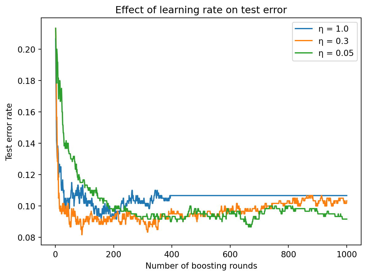
The plot shows test error as a function of boosting rounds for three learning rates. A large learning rate (\(\eta = 1.0\)) converges fast — the error drops quickly in the first few rounds — but may overshoot and plateau at a higher error or even tick upward as overfitting sets in. A small learning rate (\(\eta = 0.05\)) starts slowly and needs many more rounds to converge, but often reaches a lower final error because each step is small and careful.
The general rule in practice is: small \(\eta\) + many trees beats large \(\eta\) + few trees. A learning rate of 0.01 to 0.1 combined with hundreds or thousands of rounds typically outperforms a learning rate of 1.0 with a handful of rounds. The small learning rate acts as a regularizer — by making each tree’s contribution small, it prevents any single tree from having too much influence on the ensemble, similar to how a small step size in gradient descent prevents overshooting the minimum.
This creates a tradeoff between accuracy and computation. A smaller learning rate needs more trees to reach convergence, which means more computation. In practice, you pick a learning rate in the range 0.01–0.3 and then use cross-validation to determine how many rounds (trees) to run before overfitting sets in.
5.4 Gradient Boosting in Python
from sklearn.ensemble import GradientBoostingClassifier
from sklearn.datasets import make_classification
from sklearn.model_selection import train_test_split

# Generate data
X_gb, y_gb = make_classification(
    n_samples=500, n_features=10, n_informative=5,
    random_state=42
)
X_gb_train, X_gb_test, y_gb_train, y_gb_test = train_test_split(
    X_gb, y_gb, test_size=0.3, random_state=42
)

# Train Gradient Boosting
gb = GradientBoostingClassifier(
    n_estimators=200,      # number of boosting rounds
    learning_rate=0.1,     # step size
    max_depth=3,           # shallow trees
    random_state=42
)
gb.fit(X_gb_train, y_gb_train)

print(f"Training accuracy: {gb.score(X_gb_train, y_gb_train):.3f}")
print(f"Test accuracy: {gb.score(X_gb_test, y_gb_test):.3f}")
Training accuracy: 1.000
Test accuracy: 0.920Notice the hyperparameter choices. n_estimators=200 means we run 200 boosting rounds. learning_rate=0.1 means each tree contributes 10% of its full prediction. max_depth=3 means each tree can have at most 3 levels of splits — so each tree can capture up to 3-way interactions between features, but no more. These are reasonable defaults for a first model. In practice, you’d tune these using cross-validation, particularly the interplay between learning_rate and n_estimators (lower learning rate generally needs more estimators).
5.5 XGBoost: Extreme Gradient Boosting
XGBoost (Chen & Guestrin, 2016) is an optimized implementation of gradient boosting that has become the dominant algorithm for structured/tabular data in both industry and competitions. It adds several improvements over the basic gradient boosting algorithm described above.
First, explicit regularization. Plain gradient boosting controls overfitting indirectly through the learning rate, tree depth, and number of rounds. XGBoost adds a regularization penalty directly to the objective function, penalizing trees that are too complex (too many leaves) or that make extreme predictions (large leaf values). This gives the algorithm a more principled way to trade off accuracy against complexity.
Second, computational efficiency. XGBoost uses parallelized tree construction (evaluating splits across features simultaneously), cache-aware memory access patterns, and approximate split finding for large datasets. These engineering optimizations make it substantially faster than scikit-learn’s gradient boosting implementation, especially on large datasets.
Third, built-in handling of missing values. Instead of requiring you to impute missing values before training, XGBoost learns the best direction to send missing values at each split. During training, it tries sending missing-value observations to both the left and right child and picks whichever direction reduces the loss more. This is particularly useful in finance, where missing data is common (not all companies report all fields, not all borrowers have every feature).
Fourth, column subsampling borrowed from Random Forests. In addition to the sequential tree-building of boosting, XGBoost can randomly subsample features at each tree or at each split, just like Random Forests do. This further de-correlates the trees and provides an additional regularization mechanism.
XGBoost became famous through Kaggle competitions — for several years, it won or placed in the top ranks of the majority of competitions involving structured/tabular data. It remains one of the strongest off-the-shelf models for the kind of data that’s common in finance: rows of observations, columns of features, with a mix of numeric and categorical variables.
5.6 The XGBoost Objective Function
The mathematical distinction between XGBoost and plain gradient boosting lies in the objective function. At each boosting round, XGBoost minimizes:
\[\mathcal{L} = \sum_{i=1}^{n} l\!\left(y_i,\; \hat{y}_i + h_m(x_i)\right) + \Omega(h_m)\]
The first term is the usual loss — how well the new tree \(h_m\) corrects the current ensemble’s errors. This is the same term that plain gradient boosting minimizes. The second term \(\Omega\) (Greek capital letter “omega”) is the regularization penalty, which penalizes tree complexity:
\[\Omega(h_m) = \gamma T + \frac{1}{2}\lambda \sum_{j=1}^{T} w_j^2\]
This penalty has two parts. The first part, \(\gamma T\), charges a cost for each leaf in the tree. The parameter \(\gamma\) (gamma) controls this cost: a large \(\gamma\) means it’s expensive to add leaves, so the tree stays small. A split will only be made if the reduction in loss exceeds \(\gamma\) — otherwise, it’s not worth the complexity cost. The second part, \(\frac{1}{2}\lambda \sum w_j^2\), penalizes large prediction values in the leaves, where \(w_j\) is the prediction value in leaf \(j\). The parameter \(\lambda\) (lambda) controls this penalty: a large \(\lambda\) shrinks the leaf predictions toward zero, preventing the tree from making extreme corrections. This is analogous to the L2 (ridge) penalty we saw in Lecture 5 for regression.
The regularization is what distinguishes XGBoost from plain gradient boosting. It explicitly trades off prediction accuracy against model complexity, and it does so within the optimization rather than relying solely on external controls like learning rate and early stopping. In practice, this means XGBoost can use slightly more aggressive settings (larger learning rate, deeper trees) without overfitting as easily, because the regularization penalty keeps the trees in check.
5.7 XGBoost in Python
from xgboost import XGBClassifier
from sklearn.datasets import make_classification
from sklearn.model_selection import train_test_split

# Same data as before
X_xgb, y_xgb = make_classification(
    n_samples=500, n_features=10, n_informative=5,
    random_state=42
)
X_xgb_train, X_xgb_test, y_xgb_train, y_xgb_test = train_test_split(
    X_xgb, y_xgb, test_size=0.3, random_state=42
)

# Train XGBoost
xgb = XGBClassifier(
    n_estimators=200,
    learning_rate=0.1,
    max_depth=3,
    reg_lambda=1.0,        # L2 regularization
    random_state=42
)
xgb.fit(X_xgb_train, y_xgb_train)

print(f"Training accuracy: {xgb.score(X_xgb_train, y_xgb_train):.3f}")
print(f"Test accuracy: {xgb.score(X_xgb_test, y_xgb_test):.3f}")
Training accuracy: 1.000
Test accuracy: 0.920The interface is very similar to scikit-learn’s GradientBoostingClassifier, which is intentional — XGBClassifier follows the same .fit() / .predict() / .score() API. The additional parameter reg_lambda controls the L2 regularization on leaf weights (the \(\lambda\) in the penalty term). Setting reg_lambda=1.0 is the default and provides moderate regularization. You can increase it if you’re concerned about overfitting or decrease it toward 0 if you want a less regularized model.
5.8 XGBoost Hyperparameters
XGBoost has more hyperparameters than Random Forests, which is both its strength (more control) and its weakness (more tuning required). The most important ones are:
| Parameter | What it controls | Typical range |
|---|---|---|
n_estimators |
Number of boosting rounds | 100–1000 |
learning_rate |
Step size per round (\(\eta\)) | 0.01–0.3 |
max_depth |
Depth of each tree | 3–8 |
reg_lambda |
L2 regularization on leaf weights (\(\lambda\)) | 0–10 |
subsample |
Fraction of observations per tree | 0.5–1.0 |
colsample_bytree |
Fraction of features per tree | 0.5–1.0 |
The subsample parameter randomly selects a fraction of the training observations to use for each tree, similar to bootstrap sampling in Random Forests but without replacement. The colsample_bytree parameter randomly selects a fraction of features for each tree, directly borrowed from the Random Forest idea. Both add randomness that helps prevent overfitting and de-correlates the trees.
The interplay between learning_rate and n_estimators is the most important tuning decision. A common strategy is to fix a small learning rate (say 0.05 or 0.1) and then use cross-validation with early stopping to find the right number of rounds. Early stopping monitors validation error during training and stops when the error hasn’t improved for some number of consecutive rounds — this automatically finds the point where additional trees start to overfit.
5.9 Practical Guidance: Which Method to Use?
Both Random Forests and Gradient Boosting / XGBoost are strong models for structured data, and both are widely used in finance. The choice between them comes down to practical considerations.
Random Forests are a safe default. They’re robust to hyperparameter choices — the defaults work well on most problems, so you can get a competitive model with minimal tuning. They’re easy to parallelize across multiple CPU cores because each tree is independent. They can’t overfit by adding more trees, so n_estimators is purely a computational budget decision. And they provide OOB error estimates for free. If you need a quick, reliable baseline or if you don’t have time for extensive hyperparameter tuning, start with a Random Forest.
XGBoost typically achieves higher accuracy with careful tuning. It has a higher ceiling — on many benchmarks and competitions, a well-tuned XGBoost model beats a well-tuned Random Forest. But reaching that ceiling requires tuning the learning rate, number of rounds, tree depth, and regularization parameters, ideally with cross-validation. It’s also more sensitive to hyperparameter choices: a poorly-tuned XGBoost can underperform a default Random Forest. And because the trees are built sequentially, training can’t be parallelized as easily (though XGBoost parallelizes the construction of each individual tree).
A common workflow in practice is: start with a Random Forest to establish a baseline, then try XGBoost to see if you can beat it. If XGBoost improves substantially over the Random Forest, invest time in tuning it further. If not, stick with the Random Forest — it’s simpler and more robust.
6 Summary
This chapter introduced ensemble methods — techniques for combining many models into a stronger whole. The central insight is that individual decision trees are noisy and unstable, but their noise can be averaged away if we build many trees that make different mistakes.
Random Forests use two sources of randomness to achieve this: bootstrap sampling (each tree sees a different random subset of the training observations) and feature subsampling (each split considers a different random subset of features). Together, these reduce the correlation between trees, making the averaging more effective. Random Forests are robust, require minimal tuning, can’t overfit by adding more trees, and provide free validation via OOB error. They are the go-to default for structured data.
Gradient Boosting and XGBoost take a different approach: build trees sequentially, where each new tree fits the residuals (errors) of the current ensemble. Each tree is deliberately shallow — a small, targeted correction rather than a full model. The learning rate controls how much each tree contributes, with the general rule that small steps with many trees outperforms large steps with few trees. XGBoost adds explicit regularization on tree complexity and leaf values, as well as computational optimizations that make it practical for large datasets. These methods often achieve the highest accuracy on structured data but require more careful tuning than Random Forests.
Both families of methods are among the most widely used in applied machine learning and finance. For tabular data — the kind that comes in rows and columns, like financial statements, loan applications, and trading signals — ensemble methods based on decision trees consistently rank among the top performers.
7 References
- Breiman, L. (1996). Bagging predictors. Machine Learning, 24(2), 123–140.
- Breiman, L. (2001). Random forests. Machine Learning, 45(1), 5–32.
- Chen, T. & Guestrin, C. (2016). XGBoost: A scalable tree boosting system. Proceedings of KDD, 785–794.
- Freund, Y. & Schapire, R. E. (1997). A decision-theoretic generalization of on-line learning and an application to boosting. Journal of Computer and System Sciences, 55(1), 119–139.
- Friedman, J. H. (2001). Greedy function approximation: A gradient boosting machine. Annals of Statistics, 29(5), 1189–1232.
- Hastie, T., Tibshirani, R., & Friedman, J. (2009). The Elements of Statistical Learning (2nd ed.). Springer.