Lecture 9: Neural Networks & Deep Learning
RSM338: Machine Learning in Finance
1 Introduction
Every model we have studied so far — linear regression, Ridge and Lasso, logistic regression, decision trees, Random Forests, XGBoost — is a specific choice of prediction function \(f_\theta\) plugged into the same general framework we introduced in Lecture 5:
\[\hat{\theta} = \arg\min_{\theta} \left\{ \sum_{i=1}^{n} \mathcal{L}(y_i, f_\theta(\mathbf{x}_i)) + \lambda \cdot \text{Penalty}(\theta) \right\}\]
In that framework, \(f_\theta\) is the prediction function (parameterized by \(\theta\)), \(\mathcal{L}\) is the loss function measuring how wrong our predictions are, and \(\lambda \cdot \text{Penalty}(\theta)\) is an optional regularization term that penalizes complex models. Linear regression uses \(f_\theta(\mathbf{x}) = \mathbf{x}^\top \boldsymbol{\beta}\) with squared-error loss and no penalty. Ridge regression uses the same \(f_\theta\) but adds an L2 penalty. Logistic regression uses \(f_\theta(\mathbf{x}) = \sigma(\mathbf{x}^\top \mathbf{w})\) with cross-entropy loss. Decision trees and their ensembles partition the feature space into piecewise-constant regions.
In every case, the parameters \(\theta\) had clear interpretations. You could look at a regression coefficient and say “\(\beta_3 = 0.5\) means a one-unit increase in \(X_3\) is associated with a 0.5-unit increase in \(Y\).” Even tree splits are interpretable: “if momentum > 0.02, go left.” This lecture we add a new row to that table:
| Lecture | Model | What \(f_\theta(\mathbf{x})\) is | Parameters \(\theta\) |
|---|---|---|---|
| 5 | Linear regression | \(\mathbf{x}^\top \boldsymbol{\beta}\) | Slopes and intercept |
| 5 | Ridge / Lasso | \(\mathbf{x}^\top \boldsymbol{\beta}\) (with penalty) | Slopes and intercept |
| 7 | Logistic regression | \(\sigma(\mathbf{x}^\top \mathbf{w})\) | Weights and bias |
| 8 | Decision trees / ensembles | Piecewise-constant regions | Split rules and leaf values |
| 9 | Neural network | A composition of layers | Thousands to billions of weights |
A neural network is just another choice of \(f_\theta\) — the same loss functions, regularization ideas, and evaluation methods all carry over. What makes it different is that \(f_\theta\) is built by composing many simple operations (layer after layer of weighted sums and nonlinear transformations), and the resulting parameters — potentially millions of them — have no individual interpretation. You cannot look at weight #4,817 and say what it “means.” The model is a black box: features go in, predictions come out.
Why would we accept this? Because the other models on our list have structural limitations. Linear regression can only learn linear relationships. Logistic regression can only learn linear decision boundaries. Decision trees partition the feature space into rectangles. Even Random Forests and XGBoost are combinations of piecewise-constant functions. Neural networks trade interpretability for flexibility: by composing many layers, they can approximate essentially any continuous function. The cost is that you lose the ability to explain why the model makes a particular prediction. This tradeoff is worth it when prediction accuracy matters more than explanation — fraud detection, algorithmic trading, pricing derivatives, processing text and images.
2 From Neurons to Networks
The building block of every neural network is a neuron (also called a unit or node). A single neuron does two things: it computes a weighted sum of its inputs plus a bias term, and then applies a nonlinear function (called an activation function) to the result:
\[a = g\!\left(\sum_{j=1}^{p} w_j x_j + b\right) = g(\mathbf{w}^\top \mathbf{x} + b)\]
Here \(x_1, x_2, \ldots, x_p\) are the inputs (our features), \(w_1, w_2, \ldots, w_p\) are the weights controlling how much each input contributes, \(b\) is the bias (an offset, like an intercept in regression), and \(g(\cdot)\) is the activation function that introduces nonlinearity.
The weighted sum \(\mathbf{w}^\top \mathbf{x} + b\) should look familiar — it is the same linear combination from logistic regression. If we choose the sigmoid as our activation function, a single neuron is logistic regression:
\[a = \sigma(\mathbf{w}^\top \mathbf{x} + b) = \frac{1}{1 + e^{-(\mathbf{w}^\top \mathbf{x} + b)}}\]
If we choose no activation function at all (the “identity” activation, \(g(z) = z\)), a single neuron is just linear regression: \(\hat{y} = \mathbf{w}^\top \mathbf{x} + b\). So neural networks are not a departure from what we have learned — they are a generalization. The models we already know are special cases of a single neuron with particular activation choices.
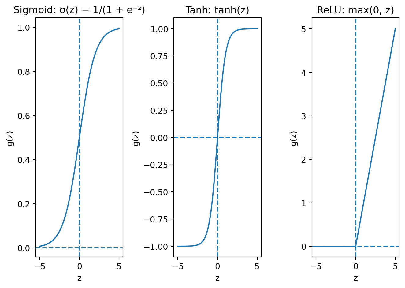
The activation function \(g\) controls what kind of nonlinearity each neuron introduces. The three most common choices are:
Sigmoid squashes any input to the range (0, 1). Look at the left panel: for very negative inputs, the output is close to 0; for very positive inputs, it is close to 1; and in between, it transitions smoothly. This is the same function from logistic regression, and it is used primarily for binary classification output layers where we need a probability. Its downside is that it suffers from vanishing gradients in deep networks — we will see why shortly. The intuition is visible in the plot: the curve is nearly flat for large positive or negative inputs, meaning the derivative is near zero in those regions. If a neuron’s input lands in one of those flat zones, the gradient signal essentially dies.
Tanh (hyperbolic tangent) squashes to the range (−1, 1). The shape is similar to sigmoid but centred at zero, which matters because it means the outputs of a tanh layer have mean roughly zero. This is better for hidden layers because the next layer receives inputs that are balanced around zero rather than always positive (as with sigmoid). When all inputs to a layer are positive, the gradients for that layer’s weights are constrained to all be the same sign, which forces the optimizer to zigzag rather than move directly toward the optimum. Centring at zero avoids this problem. But tanh still has the vanishing gradient issue — the curve flattens at the extremes, just like sigmoid.
ReLU (Rectified Linear Unit) is defined as \(g(z) = \max(0, z)\). It is the modern default for hidden layers, and looking at the right panel, you can see why it is so different from the other two. For positive inputs, ReLU is just the identity — the output equals the input, with a constant gradient of 1. For negative inputs, the output is exactly zero. This simplicity is its strength: it is computationally cheap (just a comparison and a max), and for positive inputs the gradient passes through without any shrinkage, which avoids the vanishing gradient problem that plagues sigmoid and tanh. The downside is the “dead neuron” problem: if a neuron’s weighted sum \(\mathbf{w}^\top \mathbf{x} + b\) is negative for every training example, the output is always zero, the gradient is always zero, and the weights never update. That neuron is permanently dead. In practice, this is rarely a catastrophic problem — with random initialization, most neurons start with some positive activations — but it is worth knowing about.
Why does the choice of activation function matter so much? Because it determines the fundamental character of the nonlinearity that makes neural networks powerful. If we think of each neuron as a filter that transforms its input, the activation function determines what kind of filter it is. Sigmoid and tanh are “soft” filters that smoothly compress their inputs; ReLU is a “hard” filter that either passes its input through unchanged or blocks it entirely. The hard on/off behaviour of ReLU turns out to be surprisingly effective — it creates piecewise-linear functions that can approximate complex curves through the combination of many neurons, each “turning on” at a different threshold.
But why are activation functions so critical? Without them, stacking layers does not help at all. To see why, suppose we have two layers of linear transformations with no activation:
\[\text{Layer 1: } \mathbf{h} = \mathbf{W}_1 \mathbf{x} + \mathbf{b}_1\] \[\text{Layer 2: } \hat{y} = \mathbf{W}_2 \mathbf{h} + \mathbf{b}_2\]
Substituting layer 1 into layer 2:
\[\hat{y} = \mathbf{W}_2 (\mathbf{W}_1 \mathbf{x} + \mathbf{b}_1) + \mathbf{b}_2 = \underbrace{(\mathbf{W}_2 \mathbf{W}_1)}_{\mathbf{W}'} \mathbf{x} + \underbrace{(\mathbf{W}_2 \mathbf{b}_1 + \mathbf{b}_2)}_{\mathbf{b}'}\]
This is still a linear function of \(\mathbf{x}\). No matter how many linear layers we stack, the result is always equivalent to a single linear transformation. The depth buys us nothing — two layers, ten layers, a hundred layers, the output is still just \(\mathbf{W}' \mathbf{x} + \mathbf{b}'\) for some single weight matrix and bias. Activation functions break this collapse. When we insert \(g\) between layers:
\[\hat{y} = \mathbf{W}_2 \, g(\mathbf{W}_1 \mathbf{x} + \mathbf{b}_1) + \mathbf{b}_2\]
the nonlinearity \(g\) prevents us from simplifying. Each layer now genuinely transforms the representation in a way that cannot be absorbed into a single linear operation. This is why depth matters — but only with nonlinear activations.
A single neuron is limited — it computes one number from its inputs. To get a richer transformation, we group many neurons together into a layer. A layer is a collection of neurons that all receive the same inputs but have different weights. Each neuron in the layer is looking at the same features, but each one is looking for a different pattern — one might respond strongly to high values of feature 3, another to a particular combination of features 1 and 7. Think of it like a panel of analysts who all receive the same market data but each focuses on a different signal.
With \(d\) neurons and \(p\) input features, the whole layer can be written as one matrix operation:
\[\mathbf{h} = g(\mathbf{W}\mathbf{x} + \mathbf{b})\]
where \(\mathbf{W}\) is a \(d \times p\) weight matrix (row \(k\) contains the weights for neuron \(k\)), \(\mathbf{b}\) is a \(d \times 1\) bias vector (one bias per neuron), \(g\) is applied element-wise to each neuron’s output, and \(\mathbf{h}\) is the \(d \times 1\) output vector — one value per neuron. The matrix notation is compact, but it is just a shorthand for computing \(d\) separate weighted sums in parallel and applying the activation function to each one.
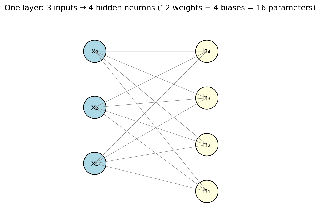
Each line in the diagram represents one weight. With 3 inputs and 4 neurons, that is \(3 \times 4 = 12\) weights plus 4 biases = 16 parameters. Already more than the 4 parameters in a 3-variable linear regression — and this is just a single layer with a handful of neurons. The “fully connected” label (sometimes called “dense”) means every input connects to every neuron. This is the most common layer type for tabular data, though specialized architectures for images and text use different connection patterns.
Notice what the layer is doing conceptually: it transforms the original \(p\) features into \(d\) new features (the values in \(\mathbf{h}\)). These new features are learned combinations of the originals, filtered through the nonlinear activation. You can think of each neuron as creating a new “derived feature” — like how an analyst might combine raw financial ratios into a composite risk score. The network learns which derived features are useful for the prediction task at hand.
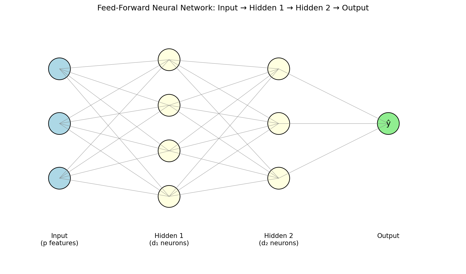
Now we get to the architecture that makes neural networks truly powerful. A feed-forward neural network (also called a multilayer perceptron or MLP) stacks layers so that each layer’s output becomes the next layer’s input:
\[\begin{align*} \mathbf{h}^{(1)} &= g\!\left(\mathbf{W}^{(1)} \mathbf{x} + \mathbf{b}^{(1)}\right) \\ \mathbf{h}^{(2)} &= g\!\left(\mathbf{W}^{(2)} \mathbf{h}^{(1)} + \mathbf{b}^{(2)}\right) \\ \hat{y} &= \mathbf{W}^{(3)} \mathbf{h}^{(2)} + \mathbf{b}^{(3)} \end{align*}\]
The intermediate outputs \(\mathbf{h}^{(\ell)}\) are called hidden layers — “hidden” because we never observe these values directly; they are internal representations that the network learns on its own. The final layer is the output layer, producing the prediction. Information flows one direction: input to hidden layers to output, with no loops or feedback.
The term “hidden” for the intermediate layers deserves a moment’s thought. In linear regression, every quantity is observable: you see the features \(\mathbf{x}\), you see the output \(\hat{y}\), and the coefficients \(\boldsymbol{\beta}\) directly relate one to the other. In a neural network, the hidden layers create intermediate representations \(\mathbf{h}^{(1)}, \mathbf{h}^{(2)}, \ldots\) that are never observed in the training data. Nobody told the network what these intermediate values should be — it learned them on its own, as a byproduct of minimizing the loss. This is one of the most remarkable aspects of deep learning: the network automatically discovers useful intermediate representations.
The depth of a network is the number of hidden layers. Modern “deep learning” models may have dozens or hundreds of layers. The term “deep learning” simply means neural networks with more than one or two hidden layers — the “deep” refers to the depth of the network, not to any philosophical profundity. But depth is not just a marketing term. Each layer transforms its input into a more abstract representation. In an image classifier, the first hidden layer might detect edges, the second layer assembles edges into shapes, and the third combines shapes into objects. Each layer builds on the representations learned by the previous one. This hierarchical feature learning is what gives deep networks their edge over shallow ones for complex data.
With the architecture in place, we need to confront a practical reality: the number of parameters grows very quickly with network size. Consider a modest example with 10 input features, a first hidden layer of 64 neurons, a second hidden layer of 32 neurons, and a single output neuron:
| Connection | Weights | Biases | Total |
|---|---|---|---|
| Input → Hidden 1 | \(10 \times 64 = 640\) | 64 | 704 |
| Hidden 1 → Hidden 2 | \(64 \times 32 = 2{,}048\) | 32 | 2,080 |
| Hidden 2 → Output | \(32 \times 1 = 32\) | 1 | 33 |
| Total | 2,817 |
Ten features and two modest hidden layers produce nearly 3,000 parameters, compared to 11 for a linear regression with the same inputs. Think about what that means: to fit a linear regression with 10 features, you need at least 11 data points to get a unique solution. To fit this neural network, you would need at least 2,817 data points just to have as many equations as unknowns — and in practice you need far more than that to avoid overfitting.
Larger architectures scale dramatically: ResNet-50, a standard image classifier, has 25 million parameters. Large language models have billions. In many neural network applications, the number of parameters far exceeds the number of training observations — a regime where OLS would not even have a unique solution (the system is underdetermined, with infinitely many perfect fits). This is one of the deep puzzles of modern deep learning: despite having far more parameters than data, well-regularized neural networks often generalize well. Managing this overparameterization — preventing the network from simply memorizing the training data — is one of the central challenges of deep learning, and it is why the regularization techniques we will cover later are so important.
The hidden layers learn a useful internal representation — they transform raw features into something more abstract and informative. The final layer translates that learned representation into the specific format our prediction task requires. This division of labour is worth emphasizing: the hidden layers are doing the hard work of feature engineering, and the output layer is just formatting the answer.
For regression (predicting a continuous value like expected returns), we use one output neuron with no activation function (the identity, \(g(z) = z\)): \(\hat{y} = \mathbf{w}^\top \mathbf{h} + b\). The output can be any real number, positive or negative, which is what we need for quantities like returns, prices, or risk measures. No activation is needed because we do not want to constrain the output range.
For binary classification (predicting default / no default), we use one output neuron with a sigmoid activation: \(\hat{y} = \sigma(\mathbf{w}^\top \mathbf{h} + b)\). The sigmoid squashes the output into the range (0, 1), which we interpret as the probability of the positive class. This is exactly logistic regression’s output, with one difference: in logistic regression, \(\hat{y} = \sigma(\mathbf{x}^\top \mathbf{w} + b)\) operates on raw features. In a neural network, \(\hat{y} = \sigma(\mathbf{h}^\top \mathbf{w} + b)\) operates on the learned hidden representation \(\mathbf{h}\). The hidden layers have already transformed the raw features into something more useful for the classification task, and the sigmoid just converts that into a probability.
For multi-class classification (predicting which of \(K\) sectors a stock belongs to, or which of \(K\) credit ratings to assign), we use \(K\) output neurons with a softmax activation:
\[\hat{y}_k = \frac{e^{z_k}}{\sum_{j=1}^{K} e^{z_j}}\]
where \(z_k\) is the raw output (called the “logit”) of neuron \(k\) before the softmax is applied. The exponential ensures all values are positive, and dividing by the sum forces them to add up to 1 — so the outputs form a proper probability distribution over the \(K\) classes. If \(z_3\) is much larger than all other \(z_k\)’s, then \(\hat{y}_3\) will be close to 1 and the rest close to 0 — the network is confidently predicting class 3. If all the \(z_k\)’s are similar, the softmax outputs will be close to \(1/K\) — the network is uncertain. Softmax is a generalization of the sigmoid: with \(K = 2\) classes, softmax reduces to exactly the sigmoid function.
Stepping back, a neural network is just a function \(f_\theta(\mathbf{x})\) that we plug into the same regression framework from Lecture 5:
\[\hat{\theta} = \arg\min_{\theta} \left\{ \sum_{i=1}^{n} \mathcal{L}\!\left(y_i, \; f_\theta(\mathbf{x}_i)\right) + \lambda \cdot \text{Penalty}(\theta) \right\}\]
What makes it different from earlier models: \(f_\theta\) is a composition of layers (weighted sums, activations, weighted sums, activations, and so on until the output); \(\theta\) contains all the weights and biases across all layers; there is no closed-form solution, so we must use iterative optimization; and the parameters have no individual interpretation. The loss \(\mathcal{L}\), the regularization penalty, the train/test split, cross-validation — all the machinery from earlier lectures carries over unchanged. The only new ingredient is the architecture of \(f_\theta\) itself.
3 The Universal Approximation Theorem
How flexible is a neural network? Could it represent any relationship between inputs and outputs? The answer is yes — with an important caveat.
The Universal Approximation Theorem (Cybenko, 1989; Hornik, 1991) states that a feed-forward neural network with a single hidden layer containing a sufficient number of neurons can approximate any continuous function on a compact domain to arbitrary accuracy. In plain language: given enough neurons, a one-hidden-layer network can get as close as you want to any smooth function.
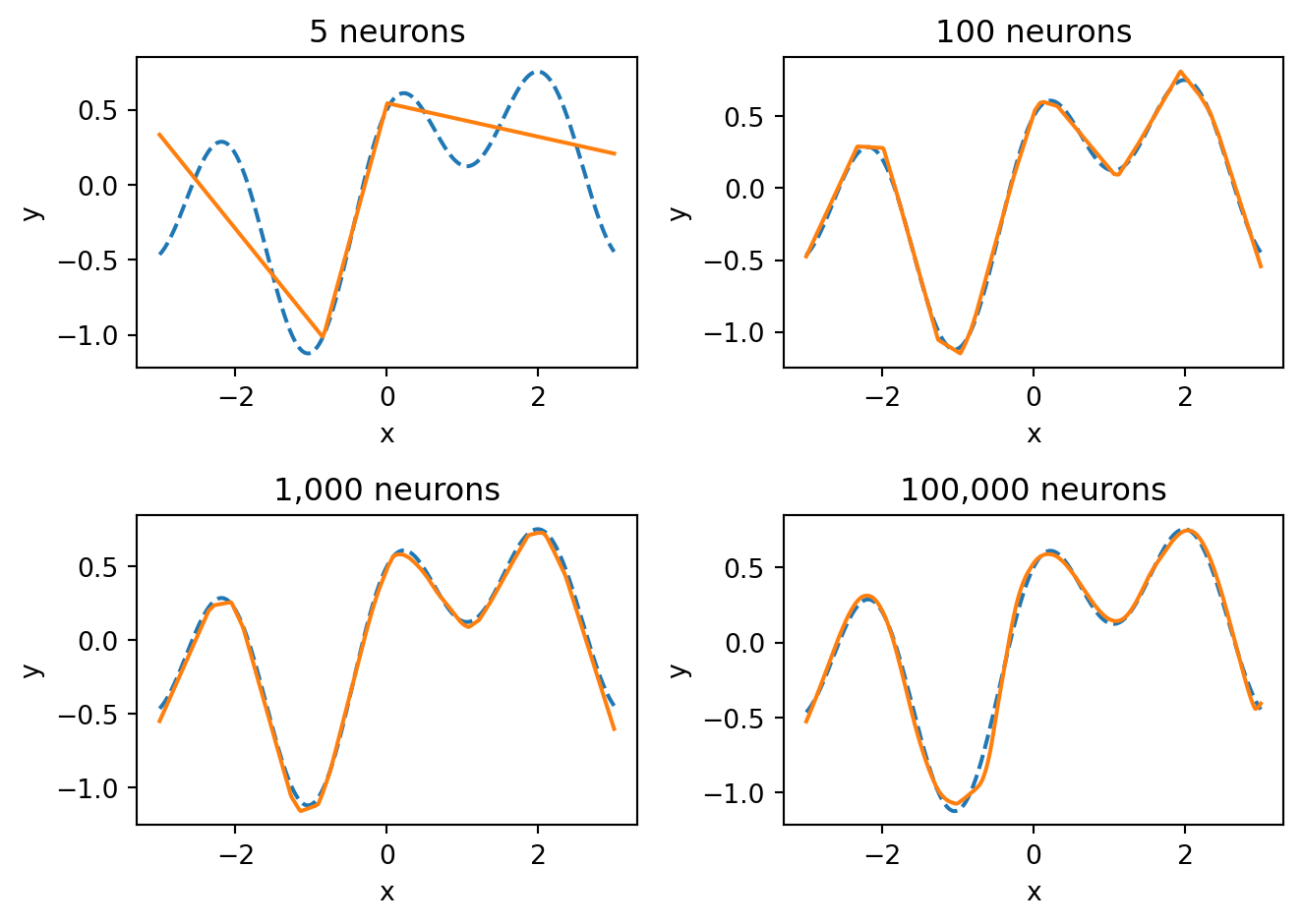
With 5 neurons, the network captures only the broad shape of the function. With 100 neurons, it gets most of the detail. With 1,000 and 100,000 neurons, the fit becomes nearly perfect — the network has enough capacity to match every wiggle of the true function. The universal approximation theorem guarantees that we can always get this close, provided we use enough neurons.
But the theorem is an existence result, not a practical guarantee. It says a solution exists; it does not say we can find it. There are several things the theorem does not promise:
That gradient descent will find the right weights. The loss landscape of a neural network is non-convex — it has many local minima and saddle points. The optimization could get stuck in a poor solution.
How many neurons you need. The theorem says “a sufficient number,” but that number could be impractically large for complex functions.
That the network will generalize. A network with enough parameters can memorize the training data perfectly (just like a high-degree polynomial can pass through every data point). The theorem says nothing about performance on new, unseen data.
That one hidden layer is the best architecture. The theorem proves one wide layer is sufficient, but in practice, deeper networks with fewer neurons per layer are more efficient. They can represent certain functions with far fewer total parameters than a single wide layer would need.
This last point is the practical motivation for “deep” learning. Depth is not about theoretical power (one layer is already enough in theory) — it is about efficiency and the ability to learn useful hierarchical representations at each level. Early layers might detect simple patterns, middle layers combine those into more complex features, and later layers assemble them into the final prediction. This hierarchical structure is what makes deep networks so effective in practice, especially for complex data like images and text.
4 Training Neural Networks
4.1 The Optimization Problem
We need to find the parameters \(\theta\) (all weights and biases across all layers) that minimize the loss:
\[\theta^* = \arg\min_{\theta} \frac{1}{n} \sum_{i=1}^{n} \mathcal{L}\!\left(y_i, \; f_\theta(\mathbf{x}_i)\right)\]
For linear regression, we had a closed-form solution: set the derivative to zero and solve. For neural networks, there is no closed-form solution. The loss is non-convex — because of the nonlinear activations, the loss landscape has many bumps, valleys, local minima, and saddle points. We cannot just solve for the optimal weights algebraically. Instead, we use gradient descent: start with random weights, compute the gradient of the loss with respect to the weights, and step in the direction that reduces the loss:
\[\theta_{t+1} = \theta_t - \eta \, \nabla_\theta \mathcal{L}\]
where \(\eta\) (the Greek letter “eta”) is the learning rate — how large a step we take at each iteration. This is the same gradient descent idea from optimization, applied to a very high-dimensional parameter space.
One of the advantages of the Lecture 5 framework is that loss functions carry over directly — we do not need to invent new ones for neural networks. The architecture of \(f_\theta\) changed, but the loss \(\mathcal{L}\) that measures prediction quality is the same.
For regression, we use mean squared error — the same loss as OLS:
\[\mathcal{L}_{\text{MSE}} = \frac{1}{n}\sum_{i=1}^{n}(y_i - \hat{y}_i)^2\]
This penalizes large errors more than small ones (because of the squaring). A prediction that is off by 10 contributes 100 to the loss, while a prediction off by 1 contributes only 1. The gradient of MSE with respect to the prediction is proportional to the error itself — \(2(y_i - \hat{y}_i)\) — which means the network gets a stronger learning signal from observations it is getting badly wrong.
For binary classification, we use binary cross-entropy — the same loss as logistic regression:
\[\mathcal{L}_{\text{BCE}} = -\frac{1}{n}\sum_{i=1}^{n}\left[y_i \log(\hat{y}_i) + (1 - y_i)\log(1 - \hat{y}_i)\right]\]
This loss is worth unpacking because its structure is clever. When the true label is \(y_i = 1\), only the first term matters: \(-\log(\hat{y}_i)\). If the model predicts \(\hat{y}_i = 0.99\) (confident and correct), the loss is \(-\log(0.99) \approx 0.01\) — almost nothing. If the model predicts \(\hat{y}_i = 0.01\) (confident and wrong), the loss is \(-\log(0.01) \approx 4.6\) — very large. The logarithm creates an asymmetry: being confidently correct is barely rewarded, but being confidently wrong is severely punished. This is exactly the behaviour we want — we want the model to be cautious about making confident predictions unless it has strong evidence. The same logic applies symmetrically when \(y_i = 0\), using the \(-\log(1 - \hat{y}_i)\) term.
For multi-class classification with \(K\) classes:
\[\mathcal{L}_{\text{CE}} = -\frac{1}{n}\sum_{i=1}^{n}\sum_{k=1}^{K} y_{ik} \log(\hat{y}_{ik})\]
where \(y_{ik} = 1\) if observation \(i\) belongs to class \(k\) and 0 otherwise. Since only one \(y_{ik}\) is 1 (the true class) and the rest are 0, this simplifies for each observation to \(-\log(\hat{y}_{i,\text{true class}})\) — the negative log of the probability the model assigned to the correct class. If the model assigns high probability to the right answer, the loss is small; if it assigns low probability to the right answer, the loss is large. This is a natural generalization of binary cross-entropy to multiple classes.
4.2 Backpropagation
With thousands or millions of parameters, how do we compute the gradient \(\nabla_\theta \mathcal{L}\)? We need the derivative of the loss with respect to every single weight in every layer. Computing this naively — perturbing each weight one at a time and measuring the change in loss — would be far too slow.
Backpropagation (Rumelhart, Hinton & Williams, 1986) solves this efficiently by exploiting the fact that a neural network is a nested composition of functions. For a 3-layer network:
\[\begin{align*} \mathbf{h}^{(1)} &= g\!\left(\mathbf{W}^{(1)} \mathbf{x} + \mathbf{b}^{(1)}\right) \\ \mathbf{h}^{(2)} &= g\!\left(\mathbf{W}^{(2)} \mathbf{h}^{(1)} + \mathbf{b}^{(2)}\right) \\ \hat{y} &= \mathbf{W}^{(3)} \mathbf{h}^{(2)} + \mathbf{b}^{(3)} \end{align*}\]
We can write the prediction as a nested composition: \(\hat{y} = f^{(3)}(f^{(2)}(f^{(1)}(\mathbf{x})))\). The chain rule from calculus lets us differentiate through each layer:
\[\frac{\partial \mathcal{L}}{\partial \mathbf{W}^{(1)}} = \underbrace{\frac{\partial \mathcal{L}}{\partial \hat{y}}}_{\text{output}} \cdot \underbrace{\frac{\partial \hat{y}}{\partial \mathbf{h}^{(2)}}}_{\text{layer 3}} \cdot \underbrace{\frac{\partial \mathbf{h}^{(2)}}{\partial \mathbf{h}^{(1)}}}_{\text{layer 2}} \cdot \underbrace{\frac{\partial \mathbf{h}^{(1)}}{\partial \mathbf{W}^{(1)}}}_{\text{layer 1}}\]
Each factor in this product involves only one layer’s local operation, which is easy to compute. The algorithm works in two passes: the forward pass computes the prediction and the loss by pushing data through the network from input to output, and the backward pass multiplies the local derivatives from right to left (output back to input) to get the gradient for every weight. Weights that contributed more to the error get larger gradient values and therefore larger updates.
Modern deep learning frameworks — PyTorch, TensorFlow, JAX — perform backpropagation automatically. You define the network architecture and the loss function; the framework handles all the derivative computation behind the scenes.
There is a catch, however. The chain rule multiplies many factors together. If each factor is small, the gradient shrinks exponentially as it travels backward through the network. Suppose each layer’s gradient contribution is around 0.25. After 4 layers: \(0.25^4 \approx 0.004\). After 10 layers: \(0.25^{10} \approx 0.000001\). The gradient signal that reaches the early layers is so tiny that those layers barely learn anything — their weights hardly change even though the loss is still high.
This is the vanishing gradient problem, and it plagued early attempts at deep learning. It happens with sigmoid and tanh activations because their gradients are always less than 1 (the sigmoid’s maximum gradient is 0.25, occurring at \(z = 0\)). Every layer multiplies the gradient by a number less than 1, and the product quickly approaches zero.
ReLU largely solves this problem. The gradient of ReLU is either 0 (for negative inputs) or 1 (for positive inputs). For positive inputs, the gradient passes through unchanged — no shrinkage. This is one of the main reasons ReLU became the default activation function for hidden layers and enabled the training of much deeper networks.
4.3 Gradient Descent in Practice
Standard gradient descent computes the gradient using the entire training set at each step. If you have a million training observations, you need to push all one million through the network, compute the loss, and backpropagate before you can take a single step. This is like reading every page of a textbook before you are allowed to update your understanding — thorough, but painfully slow.
Stochastic Gradient Descent (SGD) uses a small random subset of the data (a mini-batch) instead:
\[\theta_{t+1} = \theta_t - \eta \, \nabla_\theta \mathcal{L}_{\text{batch}}\]
The mini-batch gradient is a noisy estimate of the true gradient. On average, it points in the right direction (it is an unbiased estimator of the full gradient), but any single mini-batch might point somewhat off. Think of polling: asking 100 randomly selected voters gives you a noisy estimate of the full population’s opinion, but it is much faster than asking everyone, and the noise averages out over many polls.
This noise turns out to be a feature, not a bug. The loss landscape of a neural network is non-convex, with many local minima — shallow valleys where the optimizer could get stuck. The noise in mini-batch gradients can bounce the optimizer out of these shallow valleys, helping it find deeper, better minima that full-batch gradient descent might miss. It is as if you were navigating a hilly landscape in fog: a bit of random jostling can knock you out of a shallow ditch and into a better valley.
Common mini-batch sizes are 32, 64, 128, or 256 observations. The tradeoff: smaller batches introduce more noise per step, which helps escape bad minima but makes convergence noisier and slower. Larger batches give smoother, more accurate gradient estimates, but use more memory and may get stuck in sharp minima that generalize poorly. In practice, batch sizes of 32 or 64 are a common default.
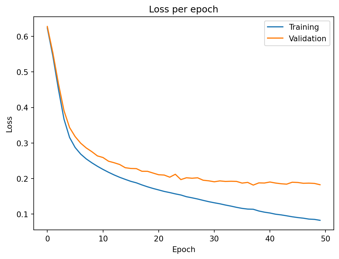
An epoch is one complete pass through the entire training set. If you have 10,000 training observations and a mini-batch size of 100, each epoch consists of 100 mini-batch updates. After one epoch, every observation has been used exactly once. Training typically runs for many epochs — the optimizer sees the same data repeatedly, refining the weights each time.
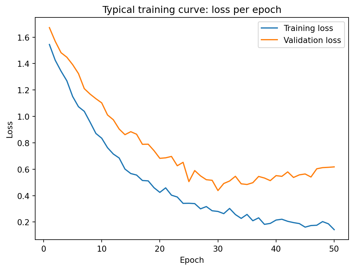
A typical training curve looks like the figure above. Training loss decreases steadily as the network fits the data better with each epoch. Validation loss decreases initially — the network is learning genuine patterns — but eventually starts to increase. This is the point where the model begins overfitting: memorizing training data noise rather than learning generalizable patterns. The growing gap between the two curves is the signal that we should stop training, which leads us to the regularization techniques discussed later.
The learning rate \(\eta\) controls how large a step the optimizer takes at each iteration. It is usually the single most important hyperparameter to get right when training a neural network.
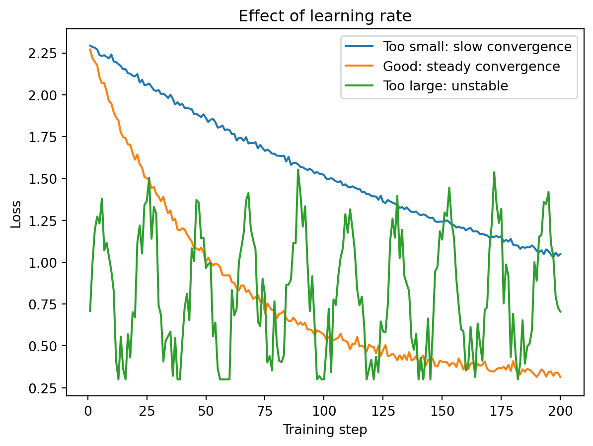
If the learning rate is too small, the model learns very slowly — you might need thousands of epochs and the training is wasteful. If the learning rate is too large, the model overshoots and bounces around the loss landscape, never settling into a good minimum. The loss oscillates wildly or even diverges. With a well-chosen learning rate, the loss decreases steadily and converges to a low value.
Typical starting values are \(\eta = 0.001\) for the Adam optimizer and \(\eta = 0.01\) for SGD. Many practitioners also reduce the learning rate during training (a technique called learning rate scheduling) so that the optimizer takes large steps initially and smaller, more precise steps as it approaches a good solution.
Plain SGD uses the same learning rate for every parameter and does not account for the history of past gradients. Modern optimizers improve on this.
SGD with Momentum adds a “velocity” term \(\mathbf{v}_t\) that accumulates past gradients:
\[\begin{align*} \mathbf{v}_t &= \gamma \, \mathbf{v}_{t-1} + \eta \, \nabla_\theta \mathcal{L} \\ \theta_{t+1} &= \theta_t - \mathbf{v}_t \end{align*}\]
The parameter \(\gamma\) (the Greek letter “gamma,” typically set to 0.9) controls how much history to keep. When the gradient consistently points in the same direction, the velocity builds up and the optimizer moves faster — like a ball rolling downhill that picks up speed on a consistent slope. When the gradients oscillate, the velocity averages out the noise and dampens the jitter.
Adam (Adaptive Moment Estimation; Kingma & Ba, 2015) goes further by tracking both the mean and the variance of past gradients, adapting the learning rate separately for each parameter:
\[\begin{align*} \mathbf{m}_t &= \beta_1 \, \mathbf{m}_{t-1} + (1 - \beta_1) \, \nabla_\theta \mathcal{L} && \text{(mean of gradients)} \\ \mathbf{v}_t &= \beta_2 \, \mathbf{v}_{t-1} + (1 - \beta_2) \, (\nabla_\theta \mathcal{L})^2 && \text{(variance of gradients)} \\ \theta_{t+1} &= \theta_t - \eta \, \frac{\hat{\mathbf{m}}_t}{\sqrt{\hat{\mathbf{v}}_t} + \epsilon} \end{align*}\]
where \(\hat{\mathbf{m}}_t\) and \(\hat{\mathbf{v}}_t\) are bias-corrected versions, and \(\epsilon\) (a tiny number like \(10^{-8}\)) prevents division by zero. The defaults are \(\beta_1 = 0.9\), \(\beta_2 = 0.999\). The division by \(\sqrt{\hat{\mathbf{v}}_t}\) is what makes Adam adaptive: parameters with large, consistent gradients get effectively smaller learning rates (preventing overshooting), while parameters with small, noisy gradients get effectively larger learning rates (helping them make progress). Adam is the default optimizer for most applications because it requires less tuning than SGD and converges faster in practice.
Putting it all together, training a neural network follows these steps:
- Choose the architecture: How many hidden layers? How many neurons per layer? What activation functions?
- Choose the loss function: MSE for regression, cross-entropy for classification.
- Choose the optimizer: Adam is usually the default starting point.
- Set hyperparameters: Learning rate, batch size, number of epochs.
- Train: Feed mini-batches through the network, compute the loss, backpropagate, update weights. Repeat for many epochs.
- Monitor: Track training and validation loss each epoch. Stop when validation loss stops improving.
- Evaluate: Test on held-out data to estimate real-world performance.
This is the same workflow as fitting any ML model — define the model, choose the loss, optimize, evaluate. The difference is that neural networks have more architectural choices and typically take longer to train.
5 Regularization
We now know how to build and train a neural network. But the parameter explosion we discussed earlier creates an urgent problem: with thousands or millions of free parameters, the network has more than enough capacity to memorize the training data, noise and all. This section covers the techniques that prevent that from happening.
Neural networks typically have far more parameters than training observations. A network with 50,000 parameters trained on 5,000 observations has, in principle, enough capacity to memorize every training example perfectly — including the noise. Without some form of regularization, training loss can approach zero while test loss remains high, meaning the model has memorized the training data rather than learning generalizable patterns.
Unlike Ridge or Lasso, where a single knob \(\lambda\) controls regularization, neural networks use a toolkit of complementary strategies. Each technique addresses overfitting from a different angle, and they are typically combined in practice. We will walk through each one.
5.1 Techniques
The simplest and often most effective regularization technique: stop training before the model overfits. We monitor validation loss during training, and when it stops improving (or starts increasing), we stop and use the weights from the best epoch.
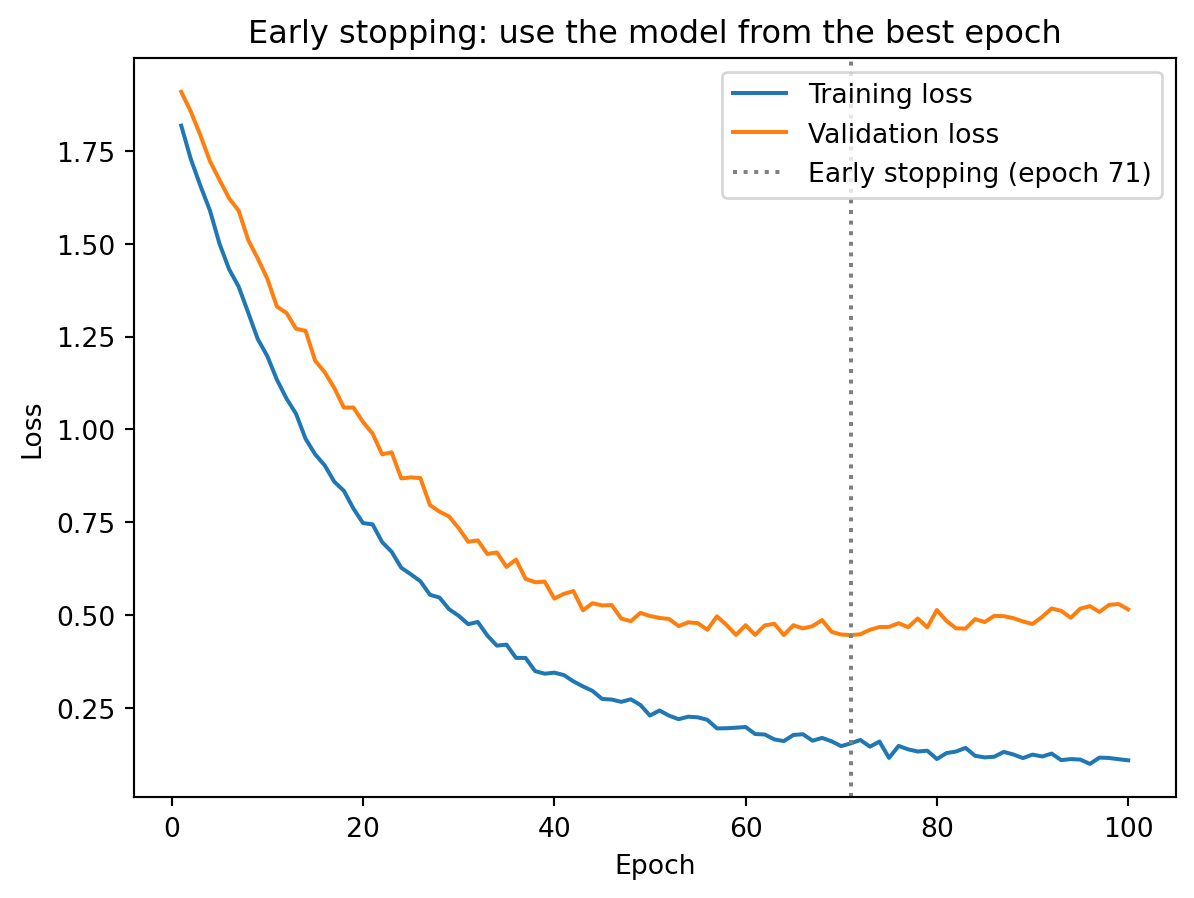
Early stopping works as implicit regularization: by limiting the number of gradient descent steps, we prevent the model from fully fitting the training noise. The logic is the same as limiting the number of boosting rounds in XGBoost — at first, each additional round improves the model on new data, but eventually the model starts fitting noise rather than signal. Stopping at the right time keeps the model in the sweet spot between underfitting and overfitting.
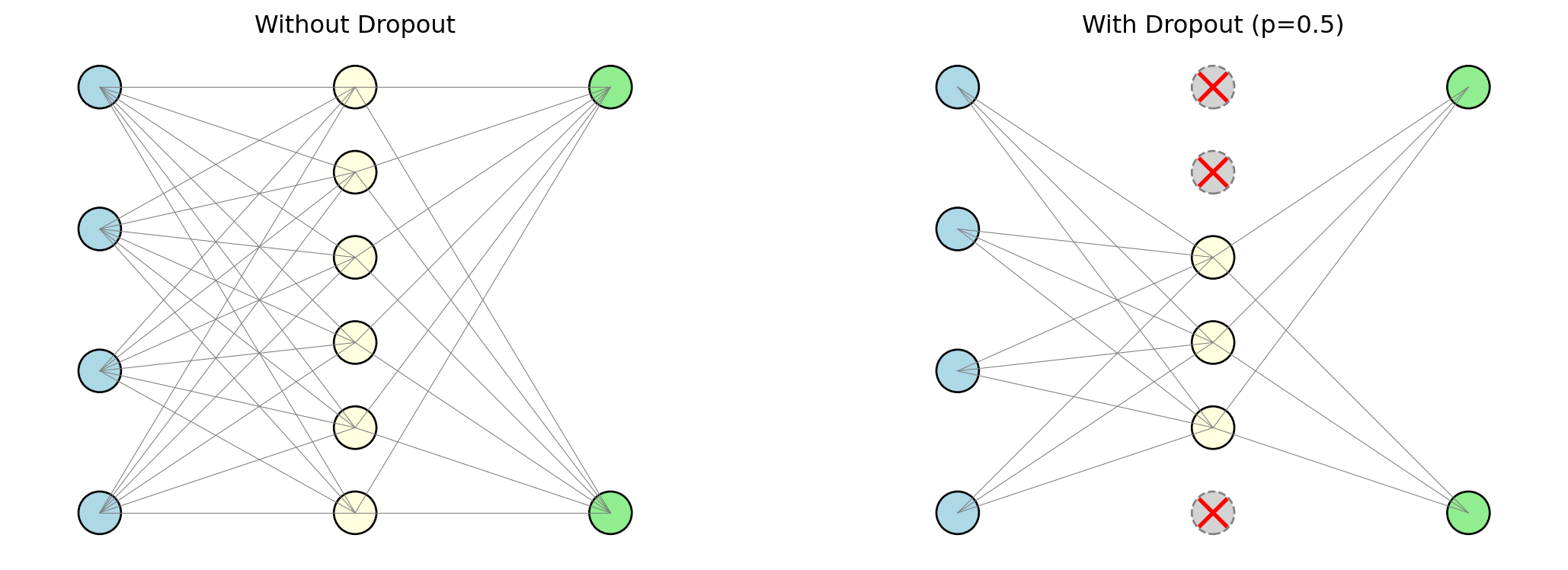
Dropout (Srivastava et al., 2014) is a regularization technique specific to neural networks, and its mechanism is wonderfully simple. During each mini-batch of training, we randomly set a fraction of the neurons to zero — effectively turning them off as if they did not exist. Each neuron is turned off independently with probability \(p\) (typically between 0.2 and 0.5). The surviving neurons must learn to make good predictions without relying on any single neuron.
Why does randomly disabling neurons help? Think about a team working on a project. If the same team member always does the critical work, the team is fragile — remove that person and the whole project falls apart. But if you randomly force team members to sit out on different days, the rest of the team must learn to cover for them. Over time, the team becomes more resilient: the knowledge and capability is distributed across everyone, not concentrated in one person. Dropout does the same thing to a neural network. Without dropout, the network can develop “co-adaptations” — configurations where a few neurons carry most of the predictive signal and the rest are parasites that only contribute in the presence of those specific neurons. Dropout breaks these co-adaptations by ensuring that no neuron can count on any other neuron being present.
One way to think about dropout is as an ensemble method built into the network. Each mini-batch trains a slightly different sub-network (whichever neurons happened to survive the random dropout), so the final trained model is effectively an average over a huge number of slightly different networks — similar to how a Random Forest averages over many slightly different trees. This prevents any small group of neurons from becoming the sole carriers of the prediction, forcing the network to distribute its knowledge more broadly.
At test time, dropout is turned off and all neurons are used. The weights are scaled to compensate for the fact that more neurons are active during testing than during any single training batch.
Weight decay applies the same L2 penalty we saw in Ridge regression (Lecture 5), but now to all the weights in a neural network:
\[\mathcal{L}_{\text{total}} = \mathcal{L}_{\text{data}} + \lambda \sum_{\ell} \|\mathbf{W}^{(\ell)}\|_2^2\]
The first term is the usual data loss (MSE or cross-entropy). The second term adds the sum of squared weights across all layers, multiplied by a penalty strength \(\lambda\). The larger \(\lambda\) is, the more the network is penalized for having large weights. At each gradient descent step, the gradient of the penalty term pulls every weight toward zero:
\[w_{t+1} = w_t - \eta \frac{\partial \mathcal{L}_{\text{data}}}{\partial w_t} - \underbrace{\eta \lambda w_t}_{\text{decay}}\]
Look at the update rule. Without the penalty, the weight update is \(w_t - \eta \cdot \text{(gradient from data)}\) — the weight moves in whatever direction reduces the data loss. With the penalty, there is an additional term \(-\eta \lambda w_t\) that pulls the weight toward zero at every step. The larger the weight, the harder it gets pulled. This is why it is called “weight decay” — the weights literally decay toward zero over time unless the data loss gradient pushes them to stay large.
Why does shrinking weights help with overfitting? A network with large weights is one that reacts intensely to its inputs — small changes in features produce large changes in predictions. This sensitivity is how the network memorizes individual training points, including their noise. A network with small weights is smoother and more moderate in its predictions, which makes it harder to overfit. The analogy to Ridge regression is exact: Ridge adds \(\lambda \|\boldsymbol{\beta}\|_2^2\) to the OLS loss, shrinking regression coefficients toward zero to prevent overfitting. Weight decay does the same thing, just with thousands of weights instead of a handful of coefficients.
As the network trains, the weights in each layer change, which means the distribution of inputs to the next layer also changes. In the first epoch, hidden layer 2 might receive inputs centred around 3 with a spread of 2. A few epochs later, after hidden layer 1’s weights have updated, the inputs to hidden layer 2 might be centred around -1 with a spread of 0.5. This constant shifting of input distributions — called internal covariate shift — makes training difficult because each layer is trying to learn on a moving target.
Batch Normalization (Ioffe & Szegedy, 2015) fixes this by normalizing each neuron’s output across the mini-batch:
\[\hat{z} = \frac{z - \mu_{\text{batch}}}{\sigma_{\text{batch}}}\]
where \(\mu_{\text{batch}}\) and \(\sigma_{\text{batch}}\) are the mean and standard deviation computed over the current mini-batch. This is the same standardization we apply to features before training (centre at zero, scale to unit variance), but applied inside the network at every layer, at every training step. After normalizing, the network learns two additional parameters per neuron — a scale \(\gamma\) and a shift \(\beta\) — so that if the normalization is harmful for some neurons, the network can learn to undo it. The result: training is more stable, higher learning rates can be used without the loss diverging, and the normalization itself acts as a mild regularizer (because each observation’s normalized value depends on the other observations in the mini-batch, introducing slight noise).
Layer Normalization (Ba, Lei & Hinton, 2016) takes a different approach: instead of normalizing across the mini-batch (computing statistics over the \(B\) observations in the batch for each neuron), it normalizes across features within each individual observation (computing statistics over the \(d\) neurons in the layer for each observation). The practical difference: batch normalization’s statistics depend on the batch size and composition, which introduces variability; layer normalization’s statistics depend only on the single observation being processed, making it more stable for small batch sizes. Layer normalization is the standard for transformer architectures, where batch sizes can vary and the model needs to handle single observations at inference time.
Finally, there are two ways to add capacity to a network: go wider (more neurons per layer) or go deeper (more layers with fewer neurons each). The universal approximation theorem tells us one wide layer is sufficient in theory. So why not just use one enormous layer?
The answer is efficiency. Consider trying to model a function that first checks whether the input is positive, then squares it if so, and takes the absolute value if not. A single wide layer can approximate this, but it might need hundreds of neurons to piece together the two different behaviours. A two-layer network can handle it naturally: the first layer separates positive from negative inputs, and the second layer applies the appropriate transformation to each group. The deep network solves the problem with far fewer total parameters because it breaks the task into stages — each layer handles one part of the logic.
This is the principle behind hierarchical representations. In an image classifier, early layers learn to detect edges (simple patterns like “there’s a vertical line here”), middle layers combine edges into shapes (“those lines form a rectangle”), and later layers combine shapes into objects (“that rectangle with those other shapes is a car”). Each layer builds on the abstractions created by the one before it. For tabular financial data, the hierarchy is less visually intuitive but still present: the first layer might learn nonlinear transformations of individual features (like a threshold effect in credit score), and the second layer might learn interactions between those transformed features (like the combination of high debt-to-income and low credit score being particularly risky).
The tradeoff is that deeper networks are harder to train. The vanishing gradient problem becomes more severe with more layers (though ReLU and batch normalization help). More layers means more hyperparameters to tune and longer training times. For tabular financial data, 2–4 hidden layers usually suffice. Networks with 50+ layers are common in computer vision and natural language processing, where the data has rich hierarchical structure that justifies the added depth.
To summarize the toolkit:
| Technique | What it does | Analogy |
|---|---|---|
| Early stopping | Stop before the model overfits | Limiting boosting rounds in XGBoost |
| Dropout | Randomly disable neurons during training | Ensemble averaging (like Random Forests) |
| Weight decay | Penalize large weights (L2 penalty) | Ridge regression’s \(\lambda \|\boldsymbol{\beta}\|_2^2\) |
| Batch / Layer norm | Normalize intermediate values | Standardizing features before regression |
In practice, these techniques are often combined. A typical setup uses ReLU activations, the Adam optimizer, dropout between 0.2 and 0.5, early stopping based on validation loss, and some weight decay.
6 Demo: Neural Networks in PyTorch
PyTorch is the most widely used deep learning framework in research and increasingly in industry. It handles all the backpropagation, gradient computation, and optimization automatically — you define the architecture and the training loop, and the framework takes care of the calculus.
We will build a simple binary classifier using synthetic data, the same kind of classification problem we tackled with Random Forests and XGBoost in previous lectures.
import numpy as np
import torch
import torch.nn as nn
from sklearn.datasets import make_classification
from sklearn.model_selection import train_test_split
from sklearn.preprocessing import StandardScaler

# Generate data
X, y = make_classification(
    n_samples=1000, n_features=10, n_informative=5,
    random_state=42
)

# Split into train, validation, and test
X_temp, X_test, y_temp, y_test = train_test_split(
    X, y, test_size=0.2, random_state=42
)
X_train, X_val, y_train, y_val = train_test_split(
    X_temp, y_temp, test_size=0.2, random_state=42
)

# Standardize features (neural networks are sensitive to feature scales)
scaler = StandardScaler()
X_train = scaler.fit_transform(X_train)
X_val = scaler.transform(X_val)
X_test = scaler.transform(X_test)

# Convert to PyTorch tensors
X_train_t = torch.tensor(X_train, dtype=torch.float32)
y_train_t = torch.tensor(y_train, dtype=torch.float32).unsqueeze(1)
X_val_t = torch.tensor(X_val, dtype=torch.float32)
y_val_t = torch.tensor(y_val, dtype=torch.float32).unsqueeze(1)
X_test_t = torch.tensor(X_test, dtype=torch.float32)
y_test_t = torch.tensor(y_test, dtype=torch.float32).unsqueeze(1)

print(f"Training set:   {X_train_t.shape[0]} observations")
print(f"Validation set: {X_val_t.shape[0]} observations")
print(f"Test set:       {X_test_t.shape[0]} observations")
Training set: 640 observations
Validation set: 160 observations
Test set: 200 observationsA few things to note about the setup. We split the data three ways: training, validation, and test. The validation set is used during training to monitor for overfitting (this is where early stopping watches); the test set is held out entirely and used only at the very end to estimate real-world performance. We also standardize the features using StandardScaler, which centres each feature at mean zero and scales it to unit variance. Neural networks are sensitive to feature scales because the gradient descent updates depend on the magnitude of the inputs — a feature measured in billions would dominate a feature measured in decimals, leading to erratic training. Standardizing puts all features on an equal footing.
With the data ready, we define the model:
# Build a feed-forward neural network
model = nn.Sequential(
    nn.Linear(10, 64),   # hidden layer 1: 64 neurons
    nn.ReLU(),
    nn.Linear(64, 32),   # hidden layer 2: 32 neurons
    nn.ReLU(),
    nn.Linear(32, 1),    # output layer: 1 neuron
    nn.Sigmoid()          # sigmoid for binary classification
)

# Choose optimizer and loss function
optimizer = torch.optim.Adam(model.parameters(), lr=0.001)
loss_fn = nn.BCELoss()  # binary cross-entropy

print(model)
print(f"\nTotal parameters: {sum(p.numel() for p in model.parameters()):,}")
Sequential(
(0): Linear(in_features=10, out_features=64, bias=True)
(1): ReLU()
(2): Linear(in_features=64, out_features=32, bias=True)
(3): ReLU()
(4): Linear(in_features=32, out_features=1, bias=True)
(5): Sigmoid()
)
Total parameters: 2,817The model is defined using nn.Sequential, which chains layers together in order. Each nn.Linear layer is a fully-connected layer (every neuron connects to every neuron in the previous layer). ReLU activations are placed between hidden layers to introduce nonlinearity. The output layer uses a sigmoid activation to produce a probability between 0 and 1. We use the Adam optimizer with a learning rate of 0.001 and binary cross-entropy as the loss function — exactly the choices we discussed in the training section.
Now we train it:
from torch.utils.data import TensorDataset, DataLoader

# Create data loader for mini-batching
train_loader = DataLoader(TensorDataset(X_train_t, y_train_t), batch_size=32, shuffle=True)

# Training loop
train_losses = []
val_losses = []

torch.manual_seed(42)

for epoch in range(50):
    # Training phase
    for X_batch, y_batch in train_loader:
        optimizer.zero_grad()           # reset gradients
        y_pred = model(X_batch)         # forward pass
        loss = loss_fn(y_pred, y_batch) # compute loss
        loss.backward()                 # backpropagation
        optimizer.step()                # update weights

    # Record losses (no gradients needed for evaluation)
    with torch.no_grad():
        train_losses.append(loss_fn(model(X_train_t), y_train_t).item())
        val_losses.append(loss_fn(model(X_val_t), y_val_t).item())

print(f"Final training loss: {train_losses[-1]:.4f}")
print(f"Final validation loss: {val_losses[-1]:.4f}")
Final training loss: 0.0821
Final validation loss: 0.1823The training loop is worth reading carefully, because it implements exactly the workflow we described earlier. The DataLoader handles mini-batching — it splits the training data into batches of 32 observations and shuffles them each epoch. For each mini-batch: optimizer.zero_grad() resets the gradients from the previous step (PyTorch accumulates gradients by default, so we need to clear them); model(X_batch) runs the forward pass to get predictions; loss_fn(y_pred, y_batch) computes the binary cross-entropy loss; loss.backward() runs backpropagation to compute gradients for every weight; and optimizer.step() updates the weights using Adam. After processing all mini-batches in an epoch, we record the training and validation losses for monitoring.
Training loss is consistently below validation loss — the model fits the training data better than unseen data, as expected. The gap between the curves is small here, indicating that the model generalizes reasonably well and is not severely overfitting. If the gap were large and growing, we would want to add regularization (dropout, weight decay) or stop training earlier.
Finally, we evaluate on the held-out test set:
# Evaluate on the held-out test set
with torch.no_grad():
    test_pred = model(X_test_t)
    test_accuracy = ((test_pred > 0.5) == y_test_t).float().mean().item()

print(f"Test accuracy: {test_accuracy:.3f}")
Test accuracy: 0.950# Compare with Random Forest and XGBoost on the same data
from sklearn.ensemble import RandomForestClassifier
from xgboost import XGBClassifier
rf = RandomForestClassifier(n_estimators=200, random_state=42)
rf.fit(X_train, y_train)
xgb = XGBClassifier(n_estimators=200, learning_rate=0.1, max_depth=3, random_state=42)
xgb.fit(X_train, y_train)
print(f"\nModel comparison on test set:")
print(f"Neural Network: {test_accuracy:.3f}")
print(f"Random Forest: {rf.score(X_test, y_test):.3f}")
print(f"XGBoost: {xgb.score(X_test, y_test):.3f}")
Model comparison on test set:
Neural Network: 0.950
Random Forest:  0.950
XGBoost:        0.945
On small tabular datasets like this one, neural networks typically perform comparably to tree-based methods — sometimes slightly better, sometimes slightly worse. The real advantage of neural networks emerges with large datasets and non-tabular data (images, text, sequences), where the ability to learn hierarchical representations from raw inputs becomes decisive. For most day-to-day financial applications involving structured tabular data (the kind of spreadsheet-format data that dominates banking, asset management, and risk analysis), XGBoost and Random Forests remain competitive and are faster to train, easier to tune, and more interpretable.
7 Neural Networks in Practice
Having covered the theory, architecture, training, and regularization, the natural question is: when should you actually use a neural network in a finance application, and when should you stick with simpler models?
Neural networks have found several niches in finance where their flexibility justifies the added complexity:
| Application | Why neural networks? |
|---|---|
| High-frequency trading | Large datasets, complex nonlinear patterns in order flow |
| Factor models | Gu, Kelly & Xiu (2020): NNs outperform linear/tree models for stock return prediction — but need large panels |
| Alternative data | Images, news, earnings calls, social media require specialized architectures (CNNs, transformers) |
| Risk management | Estimating loss distributions, stress testing, credit risk |
The Gu, Kelly & Xiu (2020) result is worth highlighting because it demonstrates the general pattern: neural networks only outperform simpler methods when there is enough data to train them. Their neural network factor model used a large panel of thousands of stocks over decades of monthly returns — a dataset where the number of observations (stock-months) is large enough to support the thousands of parameters in the network. On a smaller dataset — say, monthly returns for 50 stocks over 10 years — a simpler model like Ridge regression or XGBoost would likely perform as well or better. The lesson is not that neural networks are universally superior, but that they unlock performance gains in specific settings: large datasets, complex nonlinear relationships, and data types (text, images) that simpler models cannot handle natively.
For the vast majority of day-to-day financial analytics — credit scoring, portfolio construction, risk reporting — the data is tabular, the datasets are moderate-sized, and interpretability matters to regulators and stakeholders. In these settings, XGBoost and Random Forests remain the workhorses. Neural networks become the right tool when the dataset is large enough to support them and the problem is complex enough to reward their flexibility, or when the data itself (earnings call transcripts, satellite imagery, order book sequences) demands an architecture that can process it.
8 Beyond Feed-Forward Networks
Everything we have covered so far — neurons, layers, activations, backpropagation, regularization — applies to feed-forward networks, where information flows in one direction from input to output. But feed-forward networks process each input independently. If you feed in today’s stock features, the network has no idea what yesterday’s features were. There is no notion of order or sequence.
This is a serious limitation, because many real-world problems have richer structure than a flat vector of features. Images have spatial layout — nearby pixels are related and patterns like edges recur across the image. Time series have order — a stock that fell 5% after rising 20% is very different from a stock that fell 5% after falling 20%, even though the most recent return is identical. High-dimensional data often has low-dimensional structure hiding underneath. Specialized neural network architectures were developed to exploit each of these structures. We will not go deep into the mathematics of each architecture, but you should understand what problem each one solves and why it was designed the way it was.
8.1 Convolutional Neural Networks
A convolutional neural network (CNN) is the standard architecture for image data. It exploits a basic property of images: nearby pixels contain similar information, and the same pattern (an edge, a corner, a texture) is useful to detect regardless of where it appears.
A feed-forward network would assign one weight per pixel and connect every pixel to every neuron. For a 256×256 image, that is 65,536 weights in the first layer alone for a single neuron — and most of them would be redundant, because the same “edge detector” is useful everywhere in the image. A CNN uses weight sharing instead: a small filter (say, 3×3 pixels) slides across the entire image, applying the same weights at every position. This dramatically reduces the parameter count and prevents overfitting.
The filter slides over \(n \times n\) blocks of pixels, producing a feature map that encodes “how strongly did this pattern appear here?” Stacking many filters detects many different patterns. Multiple convolutional layers build up from simple features (edges, gradients) to increasingly complex ones (shapes, textures, objects). Because the inputs are 2D (or 3D with colour channels), the weight matrices become higher-dimensional arrays — tensors. The math generalizes from matrix multiplication to tensor operations, which becomes notationally heavy, but the core ideas are the same.
The seminal CNN architecture is LeNet-5 (LeCun, Bottou, Bengio & Haffner, 1998), designed to read handwritten cheques for banks — one of the first commercially deployed neural networks.
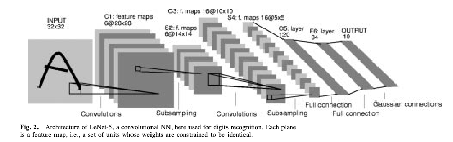
The architecture follows a pattern that became standard: input image → convolutional filters → pooling (downsampling to reduce spatial dimensions) → more convolutional filters → fully connected layers → output. The same architectural principles now power image recognition, medical imaging, and satellite analysis.
8.2 Autoencoders
An autoencoder addresses a different problem: dimensionality reduction. You have high-dimensional data (hundreds of features) but suspect that the variation is really driven by a smaller number of underlying factors. How do you find that low-dimensional structure?
A classical approach is Principal Component Analysis (PCA). PCA finds the directions of maximum variance in the data and projects onto them — compressing, say, 100 features into 5 “principal components” that capture most of the variation. It works well, but it can only find linear combinations of the original features. If the true low-dimensional structure is nonlinear (curved, folded, or otherwise complex), PCA will miss it.
An autoencoder trains a neural network to reconstruct its own input, but forces the data through a narrow bottleneck in the middle. The encoder maps the high-dimensional input down to a low-dimensional latent representation (the bottleneck) — compressing, say, 100 features into 5. The decoder maps the latent representation back up to the original dimension. The loss function is reconstruction error: how well does the output match the input? The network is never given labels — this is unsupervised learning. If the network can reconstruct the input well despite the bottleneck, the bottleneck must have learned a compressed representation that captures the essential structure. Because the encoder and decoder are neural networks with nonlinear activations, this compression can capture nonlinear relationships — it is PCA without the linearity constraint.
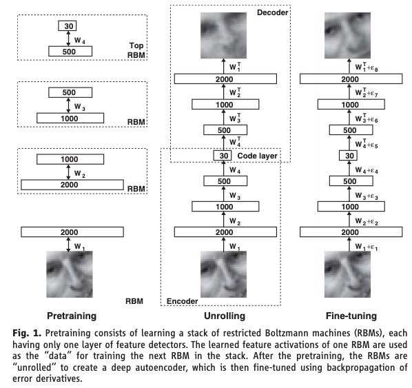
Hinton & Salakhutdinov (2006) showed that deep autoencoders dramatically outperform PCA for dimensionality reduction. This Science paper was a catalyst for the modern deep learning resurgence. A later variant, the Variational Autoencoder (VAE) by Kingma & Welling (2014), adds a probabilistic twist: instead of learning a single point in the latent space for each input, the encoder learns a distribution. This allows the decoder to generate new data by sampling from the latent space, bridging the gap between dimensionality reduction and generation.
8.3 Architectures for Sequential Data
Feed-forward networks treat each input independently. But many problems in finance are sequential — the meaning of today’s return depends on what happened yesterday, last week, and last month. An earnings call transcript is a sequence of words where order matters. A limit order book evolves through time.
A recurrent neural network (RNN) gives the network a memory. At each time step, the network receives the current input and a summary of everything it has seen so far. It produces a new hidden state that encodes everything seen up to that point, and the output prediction is computed from this hidden state. The same weights are reused at every time step — the network learns a single “update rule” that applies across the entire sequence. The seminal paper is Rumelhart, Hinton & Williams (1986): the backpropagation framework laid the foundation for training networks with recurrent connections — hidden states that feed back into themselves across time steps.
The trouble is that for long sequences, the hidden state has to carry information through many steps. In practice, the gradient signal degrades over long chains — the vanishing gradient problem again, but now in the time dimension. By the time the network reaches step 100, it has effectively forgotten what happened at step 1.
LSTM (Long Short-Term Memory; Hochreiter & Schmidhuber, 1997) fixes this by adding a separate cell state — a memory channel that runs alongside the hidden state. Think of the cell state as a conveyor belt running above the network. At each time step, three learned gates control what happens to it:
- The forget gate decides what old information to discard — “that earnings call was two quarters ago, it’s no longer relevant.”
- The input gate decides what new information to store — “this surprise Fed announcement is important, write it to memory.”
- The output gate decides what part of the memory to use for the current prediction — “for today’s forecast, the recent volatility regime matters most.”
Each gate is a small neural network that learns when to open and close from the data. The cell state can carry information forward across many time steps without degradation, because the forget gate can stay close to 1 (meaning “keep everything”) when the information is still relevant.
LSTMs became the dominant architecture for sequence modelling for nearly two decades, until transformers overtook them. They work well, but they have a fundamental bottleneck: they read sequences one token at a time, left to right. Step 50 cannot be computed until steps 1 through 49 are complete, which is slow and means that information from early in the sequence must survive through every intermediate hidden state to interact with later tokens. In language, related words can be far apart: “The executive who the board hired last quarter after a lengthy search resigned.” The subject (“executive”) and the verb (“resigned”) are nine words apart, and an RNN has to carry the memory of “executive” through all nine intermediate steps.
The transformer (Vaswani et al., 2017) takes a fundamentally different approach: throw away recurrence entirely. Instead, let every element in the sequence look at every other element directly, all at once. This mechanism is called self-attention.
Each element in the sequence (a word, a time step) gets projected into three roles:
- Query: “What am I looking for?”
- Key: “What do I have to offer?”
- Value: “Here is my actual content.”
For every pair of elements, the model computes a relevance score (how much does element A care about element B?) by comparing A’s query to B’s key. These scores become attention weights, and each element’s new representation is a weighted average of all the values in the sequence. The critical advantage is that all pairwise scores are computed simultaneously as a single matrix multiplication. This means the entire sequence is processed in parallel on a GPU, regardless of length. And any two elements can interact directly — no information needs to “survive” through intermediate steps.
“Attention Is All You Need” (Vaswani et al., 2017) is one of the most cited papers in machine learning history. Transformers are the architecture behind GPT, Claude, and every modern large language model.
8.4 Generative Models
Every model we have studied so far is discriminative — it maps inputs to a prediction. But what if you need to generate new data that looks realistic? A generative model learns to produce new data that resembles the training data.
A GAN (Generative Adversarial Network; Goodfellow et al., 2014) trains two networks against each other in a game. One tries to generate realistic fakes; the other tries to spot them. The competition drives both to improve.
- The Generator takes random noise as input and produces a synthetic data point
- The Discriminator takes a data point (either real from the training set or fake from the generator) and tries to classify it as real or fake
- They train in alternation: the discriminator gets better at detecting fakes, which forces the generator to produce more convincing fakes, which forces the discriminator to get even better, and so on
- At convergence (in theory), the generator produces data so realistic that the discriminator can’t tell the difference and guesses randomly
In practice, GAN training is notoriously unstable — the two networks can oscillate rather than converge, and the generator can collapse to producing only a few types of output. Despite this, GANs have produced remarkable results in image generation.
8.5 Diffusion Models
GANs are powerful but notoriously hard to train. The generator and discriminator can oscillate instead of converging, and the generator often suffers from mode collapse — it learns to produce only a narrow range of outputs rather than the full diversity of the training data. Diffusion models take a fundamentally different approach to generation that avoids adversarial training entirely.
The idea is to learn to reverse a gradual noising process. Start with real data and slowly add random noise over many steps until it becomes pure static. Then train a neural network to reverse each step — to take slightly noisy data and make it slightly less noisy. To generate new data, start from pure noise and apply the learned denoising steps repeatedly until a clean sample emerges.
The process has two parts. The forward process is fixed and requires no learning: take a training example \(\mathbf{x}_0\) and add a small amount of Gaussian noise at each step \(t = 1, 2, \ldots, T\). After enough steps, \(\mathbf{x}_T\) is indistinguishable from pure random noise. The reverse process is learned: a neural network \(\epsilon_\theta(\mathbf{x}_t, t)\) is trained to predict the noise that was added at each step. Given a noisy \(\mathbf{x}_t\) and the step number \(t\), the network learns to estimate what noise to subtract to recover \(\mathbf{x}_{t-1}\). To generate a new sample, draw pure noise \(\mathbf{x}_T \sim \mathcal{N}(\mathbf{0}, \mathbf{I})\) and apply the learned denoising network \(T\) times to walk back to a clean sample \(\mathbf{x}_0\).
The key advantage over GANs is stability: there is no adversarial game, so no mode collapse and no training oscillation. The trade-off is speed — generation requires many sequential denoising steps rather than a single forward pass through a generator. Diffusion models are the architecture behind DALL-E, Stable Diffusion, and modern image and video generation systems, and have largely displaced GANs as the dominant generative approach. The seminal paper is Ho, Jain & Abbeel (2020), “Denoising Diffusion Probabilistic Models.”
9 Summary
This lecture covered a lot of ground, so it is worth stepping back to see the big picture. A neural network is a choice of prediction function \(f_\theta\) — the same slot in the Lecture 5 framework that linear regression, logistic regression, and tree-based models each fill. What makes neural networks different is the architecture of that function: layers of neurons, each computing a weighted sum and passing it through a nonlinear activation, stacked so that each layer transforms the previous layer’s output into a progressively more abstract representation. The universal approximation theorem tells us this architecture can, in principle, represent any continuous function — given enough neurons. In practice, the challenge is not capacity but training: finding good weights via gradient descent, controlling overfitting through regularization, and choosing an architecture suited to the data.
For tabular financial data — the kind of structured, spreadsheet-format data that most finance professionals work with daily — neural networks compete with but rarely dominate tree-based methods like Random Forests and XGBoost. Their real advantage emerges with large datasets, complex nonlinear relationships, or non-tabular data like text and images. The specialized architectures we surveyed — CNNs for spatial data, autoencoders for dimensionality reduction, RNNs and LSTMs for sequences, transformers for long-range dependencies with parallelism, and GANs and diffusion models for generation — each extend the basic feed-forward framework by wiring the layers in a way that exploits a specific kind of structure in the data.
When you do reach for a neural network, there are more hyperparameters to manage than for any model we have studied:
| Hyperparameter | What it controls | Typical choices |
|---|---|---|
| Number of layers | Network depth | 2–4 for tabular data; dozens for images/text |
| Neurons per layer | Network width | 32, 64, 128, 256 |
| Activation function | Nonlinearity type | ReLU (hidden), sigmoid/softmax (output) |
| Learning rate | Step size in gradient descent | 0.001 (Adam), 0.01 (SGD) |
| Batch size | Observations per gradient update | 32–256 |
| Epochs | Passes through training data | Until validation loss stops improving |
| Dropout rate | Fraction of neurons dropped | 0.2–0.5 |
| Weight decay | L2 penalty strength | \(10^{-4}\) to \(10^{-2}\) |
| Optimizer | Gradient descent variant | Adam (default), SGD with momentum |
A sensible starting point: 2 hidden layers, 64 neurons each, ReLU activations, Adam optimizer with learning rate 0.001, dropout 0.3, and early stopping based on validation loss. Adjust from there based on performance.
A practical tuning strategy:
- Start simple. 2 hidden layers, 64 neurons each. Can the model overfit the training data? If training loss does not decrease, the architecture may be too small or the learning rate may be wrong.
- Get the learning rate right. If the loss barely moves, increase the learning rate. If the loss explodes or oscillates wildly, decrease it. Try \(10^{-2}\), \(10^{-3}\), and \(10^{-4}\).
- Regularize. Once you can overfit, add dropout, early stopping, and/or weight decay to close the gap between training and validation loss.
- Scale up if needed. Validation loss high and close to training loss means underfitting — go wider or deeper. Big gap between the two means overfitting — add more regularization or use a smaller network.
Some common pitfalls to watch for:
- Tuning too many things at once. Change one hyperparameter at a time. Otherwise you will not know which change helped or hurt.
- Not standardizing inputs. Feature scales matter for gradient descent. A feature in billions and one in decimals will cause erratic training. Always standardize first.
- No early stopping. The model will memorize given enough epochs. Always monitor validation loss and stop when it stops improving.
- Too deep too soon. For tabular data, 2–4 layers usually suffice. Start shallow and go deeper only if needed.
- Ignoring the baseline. Always compare against logistic regression or Random Forest. If the neural network does not beat them, the added complexity is not worth it.
- Forgetting
model.eval(). Dropout and batch normalization behave differently during training versus evaluation. Always switch the model to evaluation mode before computing test-set predictions.
10 References
- Ba, J. L., Kiros, J. R., & Hinton, G. E. (2016). Layer normalization. arXiv preprint arXiv:1607.06450.
- Cybenko, G. (1989). Approximation by superpositions of a sigmoidal function. Mathematics of Control, Signals and Systems, 2(4), 303–314.
- Goodfellow, I. J., Pouget-Abadie, J., Mirza, M., Xu, B., Warde-Farley, D., Ozair, S., Courville, A., & Bengio, Y. (2014). Generative adversarial nets. Advances in Neural Information Processing Systems, 27.
- Gu, S., Kelly, B., & Xiu, D. (2020). Empirical asset pricing via machine learning. Review of Financial Studies, 33(5), 2223–2273.
- Hastie, T., Tibshirani, R., & Friedman, J. (2009). The Elements of Statistical Learning (2nd ed.). Springer. Chapter 11.
- Hinton, G. E. & Salakhutdinov, R. R. (2006). Reducing the dimensionality of data with neural networks. Science, 313(5786), 504–507.
- Ho, J., Jain, A., & Abbeel, P. (2020). Denoising diffusion probabilistic models. Advances in Neural Information Processing Systems, 33, 6840–6851.
- Hochreiter, S. & Schmidhuber, J. (1997). Long short-term memory. Neural Computation, 9(8), 1735–1780.
- Hornik, K. (1991). Approximation capabilities of multilayer feedforward networks. Neural Networks, 4(2), 251–257.
- Ioffe, S. & Szegedy, C. (2015). Batch normalization: Accelerating deep network training by reducing internal covariate shift. Proceedings of ICML, 448–456.
- Kingma, D. P. & Ba, J. (2015). Adam: A method for stochastic optimization. Proceedings of ICLR.
- Kingma, D. P. & Welling, M. (2014). Auto-encoding variational Bayes. Proceedings of ICLR.
- LeCun, Y., Bottou, L., Bengio, Y., & Haffner, P. (1998). Gradient-based learning applied to document recognition. Proceedings of the IEEE, 86(11), 2278–2324.
- Raissi, M., Perdikaris, P., & Karniadakis, G. E. (2019). Physics-informed neural networks: A deep learning framework for solving forward and inverse problems involving nonlinear partial differential equations. Journal of Computational Physics, 378, 686–707.
- Rumelhart, D. E., Hinton, G. E., & Williams, R. J. (1986). Learning representations by back-propagating errors. Nature, 323(6088), 533–536.
- Srivastava, N., Hinton, G., Krizhevsky, A., Sutskever, I., & Salakhutdinov, R. (2014). Dropout: A simple way to prevent neural networks from overfitting. Journal of Machine Learning Research, 15, 1929–1958.
- Vaswani, A., Shazeer, N., Parmar, N., Uszkoreit, J., Jones, L., Gomez, A. N., Kaiser, L., & Polosukhin, I. (2017). Attention is all you need. Advances in Neural Information Processing Systems, 30.
More chapters coming soon