Lecture 7: Classification

RSM338: Machine Learning in Finance

Author

Kevin Mott

1 Introduction

Everything we have done so far — linear regression, ridge, lasso, cross-validation — was about predicting a continuous number. Stock returns, house prices, portfolio weights: continuous outcomes with a natural ordering. this lecture we shift to a different kind of prediction problem: classification. Instead of predicting a number, we predict a category.

Classification problems are everywhere in finance. Will a borrower default on their credit card? Is this transaction fraudulent? Will the market go up or down tomorrow? Will a firm go bankrupt in the next year? In each case the outcome is discrete — yes or no, fraud or not fraud, up or down — and the goal is to assign new observations to the correct class based on their features.

The underlying ML framework is the same: define a model, define a loss function, optimize. But the details change because the output is categorical rather than continuous. We’ll start with the most natural question — why can’t we just use regression? — and build up from there.

import numpy as np
import pandas as pd
import matplotlib.pyplot as plt

2 The Linear Probability Model

2.1 Why Not Just Use Regression?

Since we encoded default as 0/1 anyway, why not simply fit a linear regression \(\hat{y} = \beta_0 + \boldsymbol{\beta}'\mathbf{x}\) and interpret the fitted values as probabilities? This approach is called the linear probability model, and it does have a fatal flaw.

We’ll use credit card default data throughout this chapter: 1 million individuals with balance, income, and default status.

# Load credit default data
data = pd.read_csv('../Slides/credit_default.csv')

balance = data['balance'].values
income = data['income'].values
default = data['default'].values

print(f"Observations: {len(data)}")
print(f"Default rate: {default.mean():.1%}")

Observations: 1000000
Default rate: 3.3%

from sklearn.linear_model import LinearRegression

# Fit linear regression to 0/1 outcome
X = balance.reshape(-1, 1)
y = default

lr = LinearRegression()
lr.fit(X, y);

# Predict on a grid for plotting
balance_grid = np.linspace(0, 2700, 100).reshape(-1, 1)
prob_linear = lr.predict(balance_grid)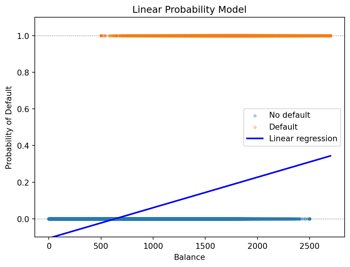

The problem is visible in the plot: linear regression produces a straight line, and that line can extend below 0 and above 1. A “probability” of \(-0.05\) or \(1.2\) doesn’t mean anything.

prob_all = lr.predict(balance.reshape(-1, 1))

print(f"Minimum predicted probability: {prob_all.min():.3f}")
print(f"Maximum predicted probability: {prob_all.max():.3f}")
print(f"Number of predictions < 0: {(prob_all < 0).sum()}")
print(f"Number of predictions > 1: {(prob_all > 1).sum()}")

Minimum predicted probability: -0.106
Maximum predicted probability: 0.344
Number of predictions < 0: 330069
Number of predictions > 1: 0

We need a function that maps any real-valued input to the interval \((0, 1)\) — a function that naturally produces valid probabilities. Logistic regression does exactly this.

3 Logistic Regression

3.1 The Logistic (Sigmoid) Function

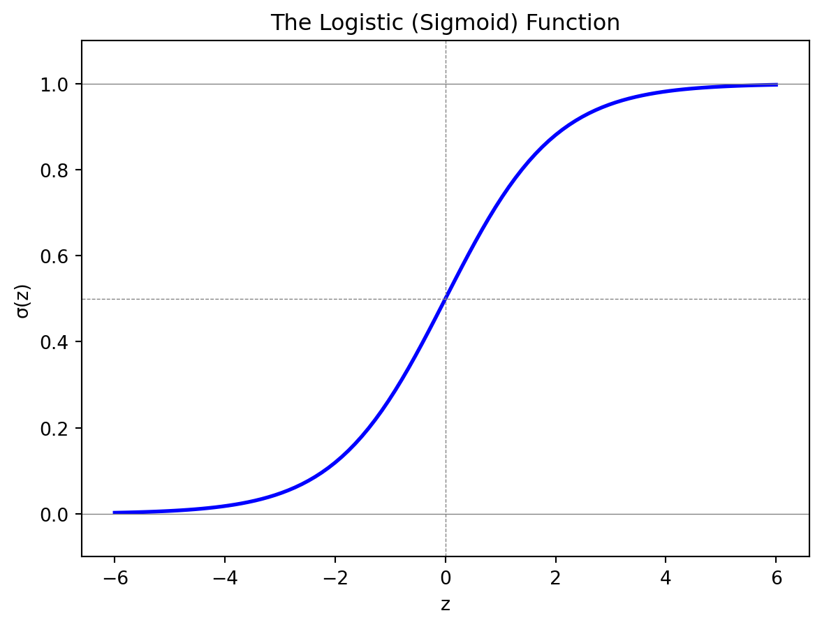
The logistic function, also called the sigmoid function, is an S-shaped curve that maps any real number to the interval \((0, 1)\):

\[\sigma(z) = \frac{e^z}{1 + e^z} = \frac{1}{1 + e^{-z}}\]

When \(z\) is very negative, \(\sigma(z)\) is close to 0. When \(z\) is very positive, \(\sigma(z)\) is close to 1. At \(z = 0\), \(\sigma(0) = 0.5\) exactly. The function is monotonically increasing — larger inputs always produce larger outputs — and it transitions smoothly between the two extremes.

3.2 The Model

In logistic regression, we model the probability of the positive class as the sigmoid applied to a linear combination of features:

\[P(y = 1 \,|\, \mathbf{x}) = \sigma(\beta_0 + \boldsymbol{\beta}' \mathbf{x}) = \frac{1}{1 + e^{-(\beta_0 + \boldsymbol{\beta}' \mathbf{x})}}\]

The notation \(P(y = 1 \,|\, \mathbf{x})\) reads “the probability that \(y = 1\) given \(\mathbf{x}\).” This is a conditional probability — the probability of default, given that we observe a particular set of feature values.

The expression inside the sigmoid, \(z = \beta_0 + \boldsymbol{\beta}'\mathbf{x} = \beta_0 + \beta_1 x_1 + \beta_2 x_2 + \cdots + \beta_p x_p\), is called the linear predictor. It can be any real number, but the sigmoid squashes it into \((0, 1)\). When \(z = 0\) the model predicts \(P(y=1) = 0.5\) (a coin flip). When \(z > 0\) the model leans toward class 1; when \(z < 0\) it leans toward class 0.

3.3 Odds and Log-Odds

To interpret logistic regression coefficients, we need the concepts of odds and log-odds.

You’ve seen odds in sports betting: “the Leafs are 3-to-1 to win” means for every 1 time they win, they lose 3 times. Formally:

\[\text{Odds} = \frac{P(\text{event})}{1 - P(\text{event})}\]

A probability of 50% corresponds to odds of 1:1 (even money). A probability of 75% gives odds of 3:1. Odds range from 0 to \(\infty\), with 1 being the neutral point.

Taking the logarithm gives us log-odds (also called the logit), which restores symmetry: log-odds of 0 means 50-50, positive means more likely than not, negative means less likely than not. In logistic regression, the log-odds is linear in the features:

\[\ln\left(\frac{P(y = 1 \,|\, \mathbf{x})}{1 - P(y = 1 \,|\, \mathbf{x})}\right) = \beta_0 + \boldsymbol{\beta}' \mathbf{x}\]

This gives us a clean interpretation of each coefficient. The coefficient \(\beta_j\) tells us how a one-unit increase in \(x_j\) changes the log-odds of the positive class. If \(\beta_j > 0\), higher \(x_j\) makes \(y = 1\) more likely. If \(\beta_j < 0\), higher \(x_j\) makes \(y = 1\) less likely. We can also convert to an odds ratio: \(e^{\beta_j}\) is the multiplicative change in odds for a one-unit increase in \(x_j\). If \(\beta_j = 0.5\), then \(e^{0.5} \approx 1.65\), meaning each one-unit increase multiplies the odds by 1.65 (a 65% increase).

3.4 The Loss Function

How do we find the best coefficients \(\beta_0, \boldsymbol{\beta}\)? The same way as any ML model: define a loss function and minimize it.

For observation \(i\) with features \(\mathbf{x}_i\) and label \(y_i\), let \(\hat{p}_i = P(y_i = 1 \,|\, \mathbf{x}_i)\) be our predicted probability. We want \(\hat{p}_i\) close to 1 when \(y_i = 1\) and close to 0 when \(y_i = 0\). The binary cross-entropy loss (also called log loss) captures this:

\[\mathcal{L}(\boldsymbol{\beta}) = -\frac{1}{n}\sum_{i=1}^{n} \left[ y_i \ln(\hat{p}_i) + (1 - y_i) \ln(1 - \hat{p}_i) \right]\]

When \(y_i = 1\), only the first term survives: the loss is \(-\ln(\hat{p}_i)\), which is small when \(\hat{p}_i\) is near 1 and very large when \(\hat{p}_i\) is near 0. When \(y_i = 0\), only the second term survives: the loss is \(-\ln(1 - \hat{p}_i)\), which penalizes predictions near 1. Cross-entropy is always non-negative and equals zero only when the model is perfectly confident and correct.

Both linear and logistic regression fit into the same ML framework — define a loss, minimize it — but with different loss functions appropriate to their outputs:

	Linear Regression	Logistic Regression
Output	Continuous \(\hat{y}\)	Probability \(\hat{p} \in (0,1)\)
Loss function	Mean squared error (MSE)	Binary cross-entropy
Formula	\(\frac{1}{n}\sum_i (y_i - \hat{y}_i)^2\)	\(-\frac{1}{n}\sum_i \left[ y_i \ln(\hat{p}_i) + (1-y_i)\ln(1-\hat{p}_i) \right]\)
Optimization	Closed-form solution	Iterative (gradient descent)

In statistics, minimizing cross-entropy is equivalent to maximum likelihood estimation. Minimizing MSE is equivalent to maximum likelihood under the assumption that errors are normally distributed. Both frameworks — ML and statistics — arrive at the same answer through different reasoning.

3.5 Fitting to the Default Data

Let’s fit logistic regression to our credit default data and compare it to the linear model.

from sklearn.linear_model import LogisticRegression

# Fit logistic regression
log_reg = LogisticRegression()
log_reg.fit(X, y);

# Predicted probabilities on the grid
prob_logistic = log_reg.predict_proba(balance_grid)[:, 1]

print(f"Intercept: {log_reg.intercept_[0]:.4f}")
print(f"Coefficient on balance: {log_reg.coef_[0, 0]:.6f}")

Intercept: -11.6163
Coefficient on balance: 0.006383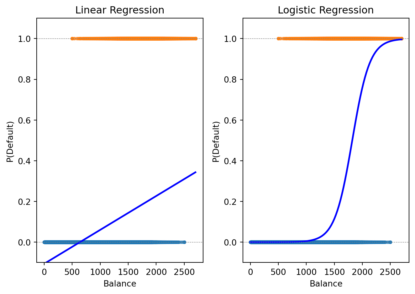

The logistic curve stays within \([0, 1]\) and captures the S-shaped relationship between balance and default probability. Where the linear model overshoots or undershoots, the logistic model produces valid probabilities.

3.6 Predictions and Thresholds

Logistic regression gives us a probability, but ultimately we need a classification — default or not. To convert probability to a class label, we choose a threshold (also called a cutoff). The default rule is to predict class 1 if \(P(y = 1 \,|\, \mathbf{x}) > 0.5\):

# Predict probabilities and apply threshold
prob_pred = log_reg.predict_proba(X)[:, 1]
class_pred = (prob_pred > 0.5).astype(int)

print(f"Using threshold = 0.5:")
print(f"  Predicted defaults: {class_pred.sum()}")
print(f"  Actual defaults: {int(default.sum())}")
print(f"  Correctly classified: {(class_pred == default).sum()} / {len(default)}")
print(f"  Accuracy: {(class_pred == default).mean():.1%}")

Using threshold = 0.5:
  Predicted defaults: 19005
  Actual defaults: 33000
  Correctly classified: 975591 / 1000000
  Accuracy: 97.6%

The 0.5 threshold is not always optimal. In a credit default setting, the cost of missing a default (false negative) is typically much higher than the cost of flagging a good borrower (false positive). We’ll return to threshold choice when we discuss evaluation metrics.

3.7 Multiple Features and Regularization

Logistic regression extends naturally to multiple predictors:

\[P(y = 1 \,|\, \mathbf{x}) = \frac{1}{1 + e^{-(\beta_0 + \beta_1 x_1 + \beta_2 x_2 + \cdots + \beta_p x_p)}}\]

# Fit with both balance and income
X_both = np.column_stack([balance, income])
log_reg_both = LogisticRegression()
log_reg_both.fit(X_both, default);

print(f"Logistic Regression with Balance and Income:")
print(f"  Intercept: {log_reg_both.intercept_[0]:.4f}")
print(f"  Coefficient on balance: {log_reg_both.coef_[0, 0]:.6f}")
print(f"  Coefficient on income: {log_reg_both.coef_[0, 1]:.9f}")

Logistic Regression with Balance and Income:
  Intercept: -11.2532
  Coefficient on balance: 0.006383
  Coefficient on income: -0.000009279

The coefficient on income is tiny — income adds very little predictive power beyond balance.

Just as with linear regression, logistic regression can overfit when there are many features. We can add regularization — lasso logistic regression adds an \(L_1\) penalty that shrinks coefficients toward zero and can perform variable selection:

\[\mathcal{L}(\boldsymbol{\beta}) - \lambda \sum_{j=1}^{p} |\beta_j|\]

The penalty \(\lambda \sum |\beta_j|\) works the same way as in lasso linear regression: it encourages sparsity by setting some coefficients exactly to zero. The regularization parameter \(\lambda\) is chosen by cross-validation.

from sklearn.linear_model import LogisticRegressionCV

# Fit Lasso logistic regression with CV
log_reg_lasso = LogisticRegressionCV(penalty='l1', solver='saga', cv=5, max_iter=1000)
log_reg_lasso.fit(X_both, default);

print(f"Lasso Logistic Regression (λ chosen by CV):")
print(f"  Best C (inverse of λ): {log_reg_lasso.C_[0]:.4f}")
print(f"  Coefficient on balance: {log_reg_lasso.coef_[0, 0]:.6f}")
print(f"  Coefficient on income: {log_reg_lasso.coef_[0, 1]:.9f}")

Lasso Logistic Regression (λ chosen by CV):
  Best C (inverse of λ): 0.0001
  Coefficient on balance: 0.001064
  Coefficient on income: -0.000123523

3.8 Multi-Class Extension

When there are \(K > 2\) classes, we generalize binary logistic regression using the softmax function. For each class \(k\), we define a separate linear predictor \(z_k = \beta_{k,0} + \boldsymbol{\beta}_k'\mathbf{x}\) and compute:

\[P(y = k \,|\, \mathbf{x}) = \frac{e^{z_k}}{\sum_{j=1}^{K} e^{z_j}}\]

This is called multinomial logistic regression or softmax regression. The softmax function ensures each probability is between 0 and 1 and that all \(K\) probabilities sum to 1. Binary logistic regression is the special case \(K = 2\).

4 Decision Boundaries

4.1 Linear Decision Boundaries

When we use logistic regression with a threshold of 0.5, we predict class 1 wherever \(P(y = 1 \,|\, \mathbf{x}) > 0.5\). The decision boundary is the set of points where the model is exactly on the fence: \(P(y = 1 \,|\, \mathbf{x}) = 0.5\).

Since \(\sigma(z) = 0.5\) when \(z = 0\), the boundary is where \(\beta_0 + \boldsymbol{\beta}'\mathbf{x} = 0\). This is a linear equation in the features, so the boundary is a straight line in 2D or a hyperplane in higher dimensions. This is why logistic regression is called a linear classifier.

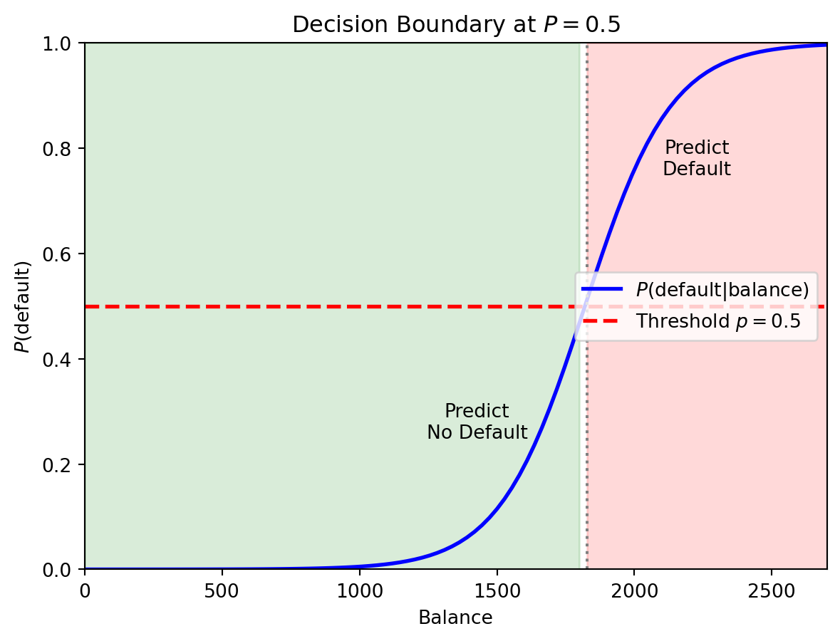
In the single-feature case the boundary is just a point on the balance axis. With two features, it’s a line in the \((x_1, x_2)\) plane that separates the “predict 0” region from the “predict 1” region.

4.2 Feature Engineering for Nonlinear Boundaries

Sometimes a straight line cannot separate the classes. Consider data where class 0 forms an inner ring and class 1 forms an outer ring — no straight line can divide them. But if we know the structure, we can add engineered features like \(x_1^2\) and \(x_2^2\). The decision boundary then becomes:

\[\beta_0 + \beta_1 x_1 + \beta_2 x_2 + \beta_3 x_1^2 + \beta_4 x_1 x_2 + \beta_5 x_2^2 = 0\]

This is a quadratic equation in the original features — it can represent circles, ellipses, or other curved shapes — even though the model is still logistic regression (linear in the expanded feature set).

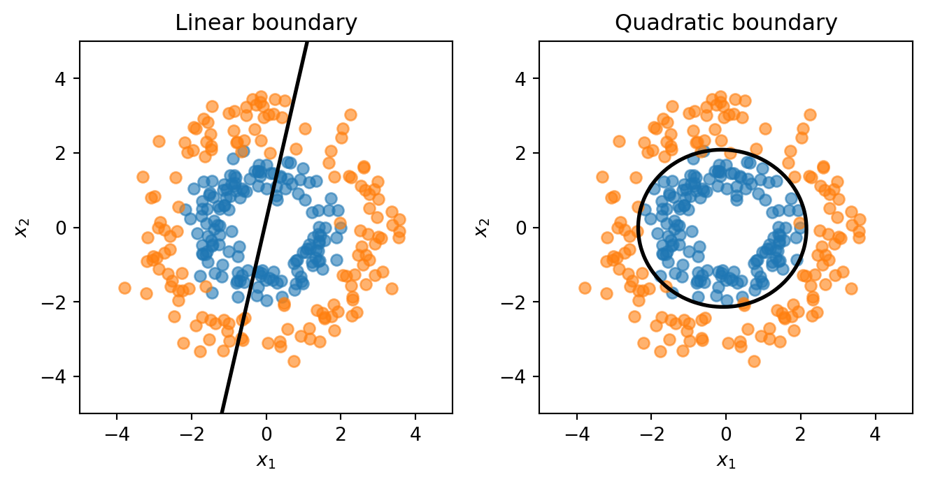
The linear model is forced to draw a straight line through the rings — hopeless. The quadratic model learns a circular boundary that actually separates the classes.

4.3 LDA and QDA

Logistic regression directly models \(P(y = 1 \,|\, \mathbf{x})\). An alternative called Linear Discriminant Analysis (LDA) takes the opposite approach: it models what each class looks like, then uses Bayes’ theorem to classify.

The idea is the same as clustering (Lecture 4), except the labels are known. LDA assumes each class follows a multivariate normal distribution \(\mathbf{x} \mid y = k \;\sim\; \mathcal{N}(\boldsymbol{\mu}_k,\, \boldsymbol{\Sigma})\), where \(\boldsymbol{\mu}_k\) is the mean of class \(k\) and \(\boldsymbol{\Sigma}\) is a shared covariance matrix across all classes. Given a new observation, we ask: which class’s distribution is it most likely to have come from?

Bayes’ theorem turns this into a scoring rule. The discriminant function for class \(k\) is:

\[\delta_k(\mathbf{x}) = \mathbf{x}' \boldsymbol{\Sigma}^{-1} \boldsymbol{\mu}_k - \frac{1}{2}\boldsymbol{\mu}_k' \boldsymbol{\Sigma}^{-1} \boldsymbol{\mu}_k + \ln \pi_k\]

where \(\pi_k = P(y = k)\) is the prior probability (the fraction of training data in class \(k\)). We classify to whichever class has the highest \(\delta_k\). Because \(\delta_k\) is linear in \(\mathbf{x}\), the decision boundary between any two classes is a straight line — just like logistic regression. No optimization loop or gradient descent is needed: LDA computes its parameters in closed form from the class means, the pooled covariance matrix, and the class proportions.

Quadratic Discriminant Analysis (QDA) relaxes the shared-covariance assumption: each class gets its own covariance matrix \(\boldsymbol{\Sigma}_k\). This introduces quadratic terms in the discriminant function, so the decision boundary between classes becomes curved.

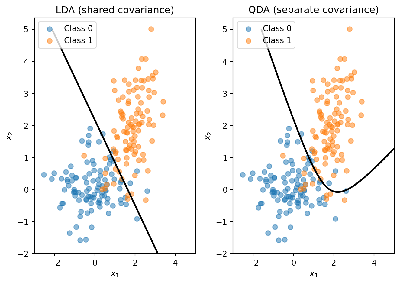
The trade-off is the usual bias-variance one. LDA has fewer parameters (one shared covariance matrix), so it’s more stable and less prone to overfitting. QDA has more parameters (one covariance matrix per class), so it’s more flexible but needs more data. When the covariance structures genuinely differ across classes, QDA can outperform LDA; when they’re similar, the extra flexibility of QDA just adds noise.

4.4 The Feature Engineering Problem

The ring example worked because we knew the right transformation — add squared terms and the circular boundary falls out. But that approach has a fundamental limitation: we have to know which transformations to use.

With 2 features, adding squares and interactions is manageable. With 50 features, there are 1,275 pairwise interactions and 50 squared terms — and there’s no guarantee that quadratic terms are the right choice. Maybe the boundary depends on \(\log(x_3)\), or \(x_7 / x_{12}\), or some transformation we’d never think to try.

We want methods that can learn nonlinear boundaries directly from the data, without us having to guess the right feature transformations in advance. These are nonparametric methods: unlike parametric models (logistic regression, LDA) which assume a specific functional form and estimate a fixed set of parameters, nonparametric models let the data determine the shape of the decision boundary.

	Parametric	Nonparametric
Structure	Fixed form (e.g., linear)	Flexible, data-driven
Parameters	Fixed number	Grows with data
Examples	Logistic regression, LDA	k-NN, Decision Trees
Risk	Bias if form is wrong	Overfitting with limited data

The next two sections cover two nonparametric classifiers: k-Nearest Neighbors and decision trees.

5 k-Nearest Neighbors

5.1 The Idea

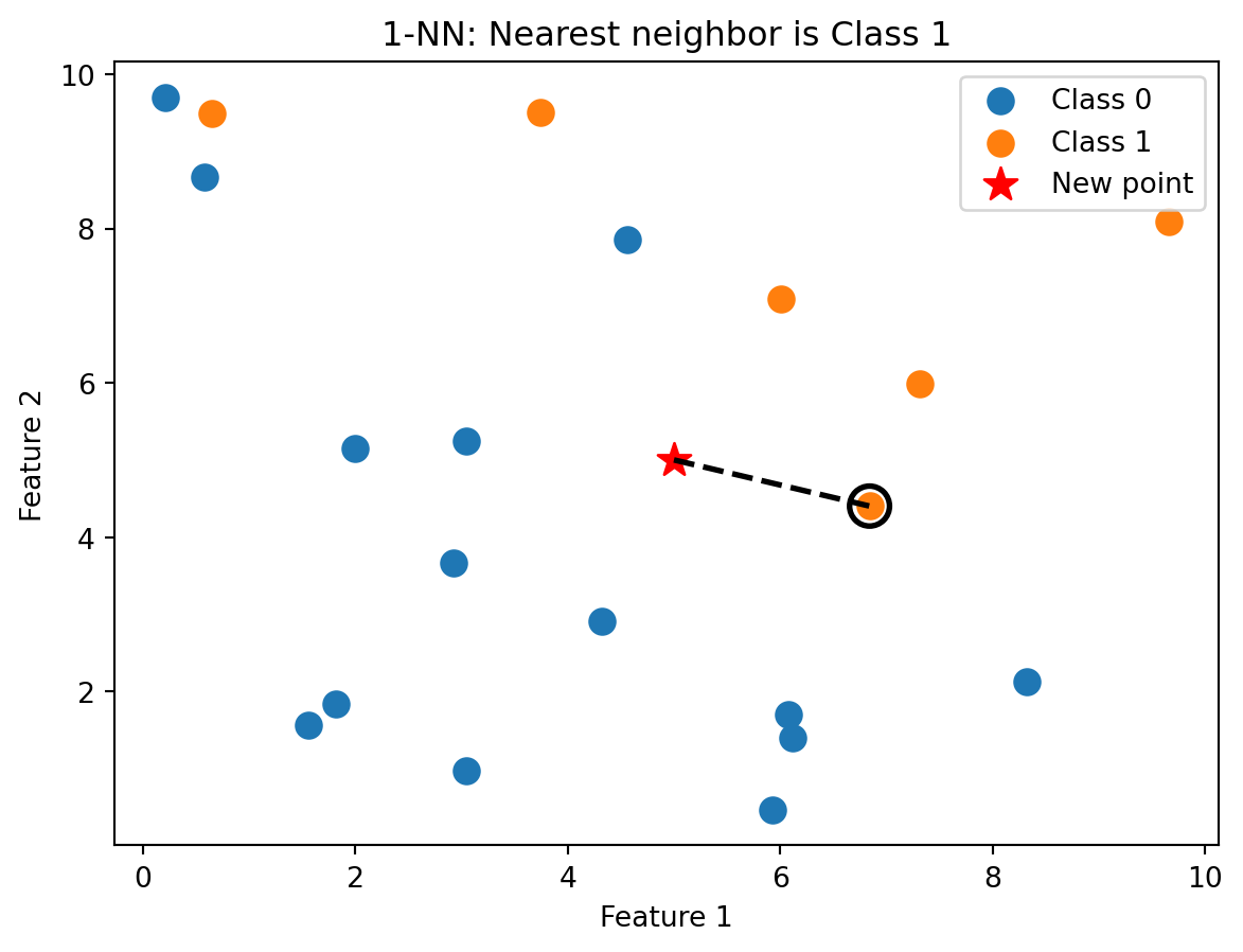
k-Nearest Neighbors (k-NN) is based on a simple idea: similar observations should have similar outcomes. To classify a new observation, find the \(k\) training observations closest to it, take a vote among those neighbours, and assign the majority class.

If you want to know whether a new loan applicant will default, look at the applicants in the training data who are most similar to them. If most of those similar applicants defaulted, predict default.

There is no training phase in the usual sense — k-NN stores all the training data and does the work at prediction time. This is sometimes called a lazy learner. The algorithm is:

Compute the distance from the new observation \(\mathbf{x}\) to every training observation \(\mathbf{x}_i\)
Identify the \(k\) training observations with the smallest distances — call this set \(\mathcal{N}_k(\mathbf{x})\)
Assign the class that appears most frequently among the \(k\) neighbours:

\[\hat{y} = \arg\max_c \sum_{i \in \mathcal{N}_k(\mathbf{x})} \mathbb{1}_{\{y_i = c\}}\]

The notation \(\mathbb{1}_{\{y_i = c\}}\) is the indicator function: it equals 1 if \(y_i = c\) and 0 otherwise. We’re just counting votes.

5.2 Distance

k-NN needs to measure how “close” two observations are. This is the same notion of distance we used in clustering (Lecture 4):

\[d(\mathbf{x}_i, \mathbf{x}_j) = \|\mathbf{x}_i - \mathbf{x}_j\| = \sqrt{\sum_{k=1}^{p} (x_{ik} - x_{jk})^2}\]

Two reminders from Lecture 4. First, standardize features before computing distances. Features on different scales (income in dollars vs. debt-to-income ratio as a percentage) will make distance meaningless — the feature with the largest scale will dominate. Standardize each feature to mean 0 and standard deviation 1 before applying k-NN. Second, the \(L_2\) (Euclidean) norm is the default choice. Manhattan (\(L_1\)) distance is an alternative, but Euclidean works well for most applications.

5.3 Visualizing k-NN

With \(k = 1\), we classify based on the single closest training point. The new observation gets assigned the class of its nearest neighbour.

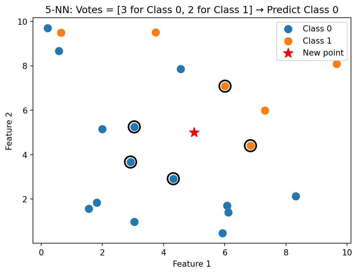
With \(k = 5\), we take a majority vote among the five nearest neighbours. This is more robust than relying on a single point, which could be noisy.

Unlike logistic regression, k-NN doesn’t compute a decision boundary explicitly. But we can visualize what the boundary looks like by classifying every point in the feature space:

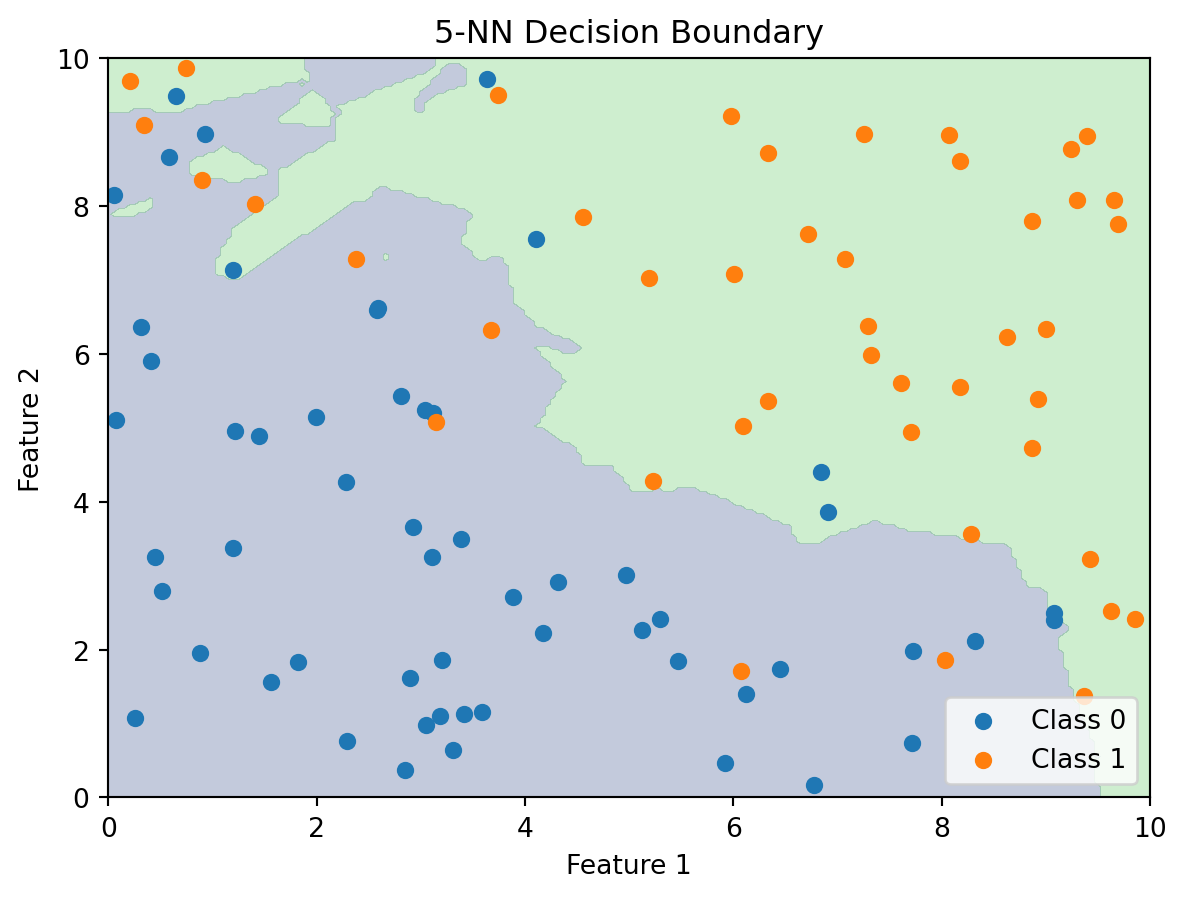
The k-NN decision boundary is nonlinear and adapts to the local density of data. It naturally forms complex shapes without us specifying any functional form.

5.4 The Role of k

The choice of \(k\) controls the bias-variance tradeoff:

Small \(k\) (e.g., \(k = 1\)): The boundary closely follows the training data, capturing complex local patterns. But it’s highly sensitive to noise. A single mislabelled point creates its own island in the decision boundary. This is high variance, low bias — the model is flexible but unstable.
Large \(k\) (e.g., \(k = 100\)): The boundary is smooth because each prediction averages over many neighbours. Local patterns get washed out. This is low variance, high bias — the model is stable but may miss real structure.

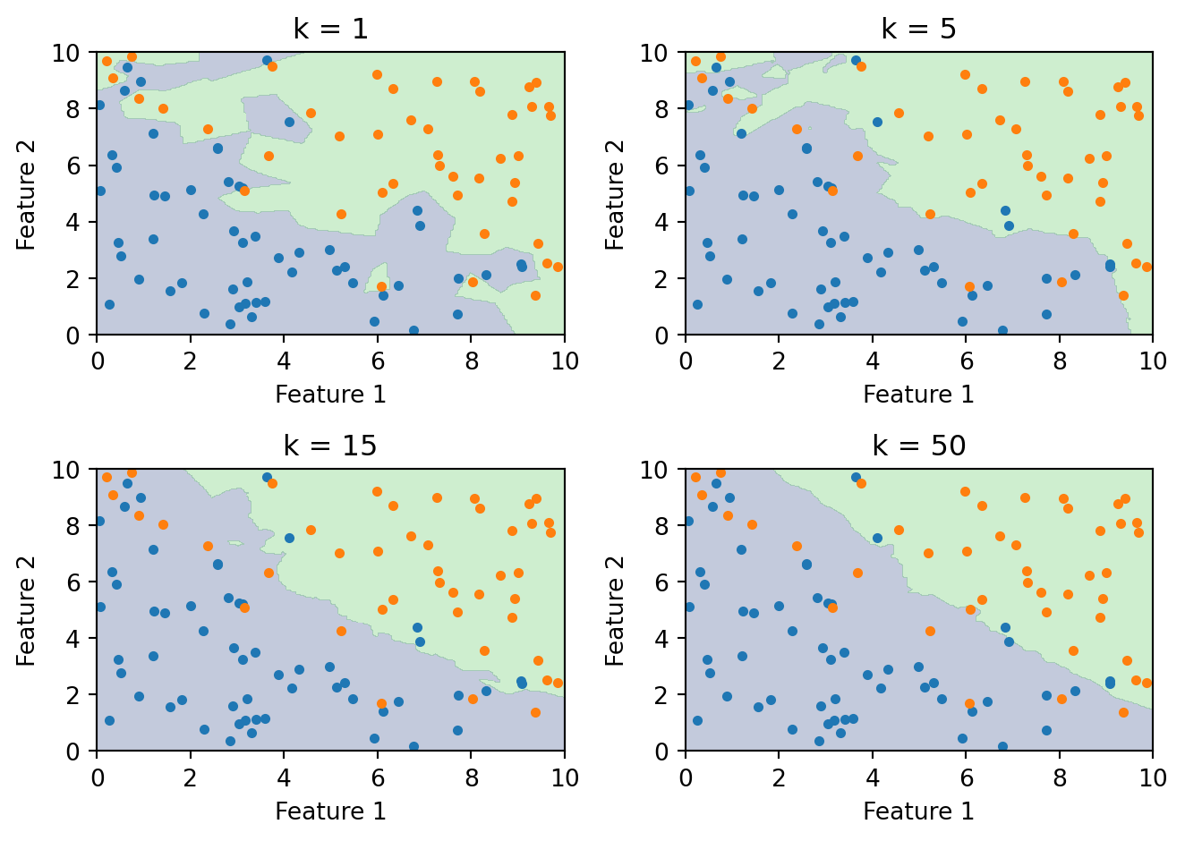
As \(k\) increases from 1 to 50, the boundary goes from jagged (overfitting) to smooth (approaching the overall majority class). The right \(k\) balances these two extremes.

We choose \(k\) by cross-validation, just as we chose the regularization parameter \(\lambda\) in Lecture 5:

from sklearn.neighbors import KNeighborsClassifier
from sklearn.model_selection import cross_val_score

k_values = range(1, 31)
cv_scores = []

for k in k_values:
    knn = KNeighborsClassifier(n_neighbors=k)
    scores = cross_val_score(knn, X_train, y_train, cv=5)
    cv_scores.append(scores.mean())

best_k = k_values[np.argmax(cv_scores)]
print(f"Best k: {best_k} with CV accuracy: {max(cv_scores):.3f}")

Best k: 19 with CV accuracy: 0.850

5.5 The Curse of Dimensionality

k-NN relies on distance, and distance breaks down in high dimensions. There are three related problems.

First, the space becomes sparse. In one dimension, 100 points cover a line segment well. In two dimensions, those same 100 points are scattered across a plane. In 50 dimensions, they’re lost in a vast empty space. The amount of data needed to “fill” a space grows exponentially with the number of dimensions.

Second, you need more data to have local neighbours. If the space is mostly empty, the \(k\) “nearest” neighbours may actually be far away — and far-away neighbours aren’t informative about local structure.

Third, distances become less informative. Euclidean distance sums \(p\) squared differences. As \(p\) grows, all these sums converge to roughly the same value (by the law of large numbers). The nearest and farthest neighbours end up almost equidistant, so “nearest” stops meaning much.

These issues make k-NN less practical when the number of features is large. In finance, where datasets often have dozens or hundreds of features, this is a real concern. Dimensionality reduction or feature selection before applying k-NN can help.

5.6 Strengths and Limitations

k-NN is simple to understand and implement, naturally handles multi-class problems, requires no distributional assumptions, and can capture arbitrarily complex boundaries. But it’s slow at prediction time (it must compute distances to every training point), sensitive to irrelevant features (which pollute the distance calculation), and struggles in high dimensions. It also requires feature scaling, since features on different scales will dominate the distance computation.

6 Decision Trees

6.1 The Idea

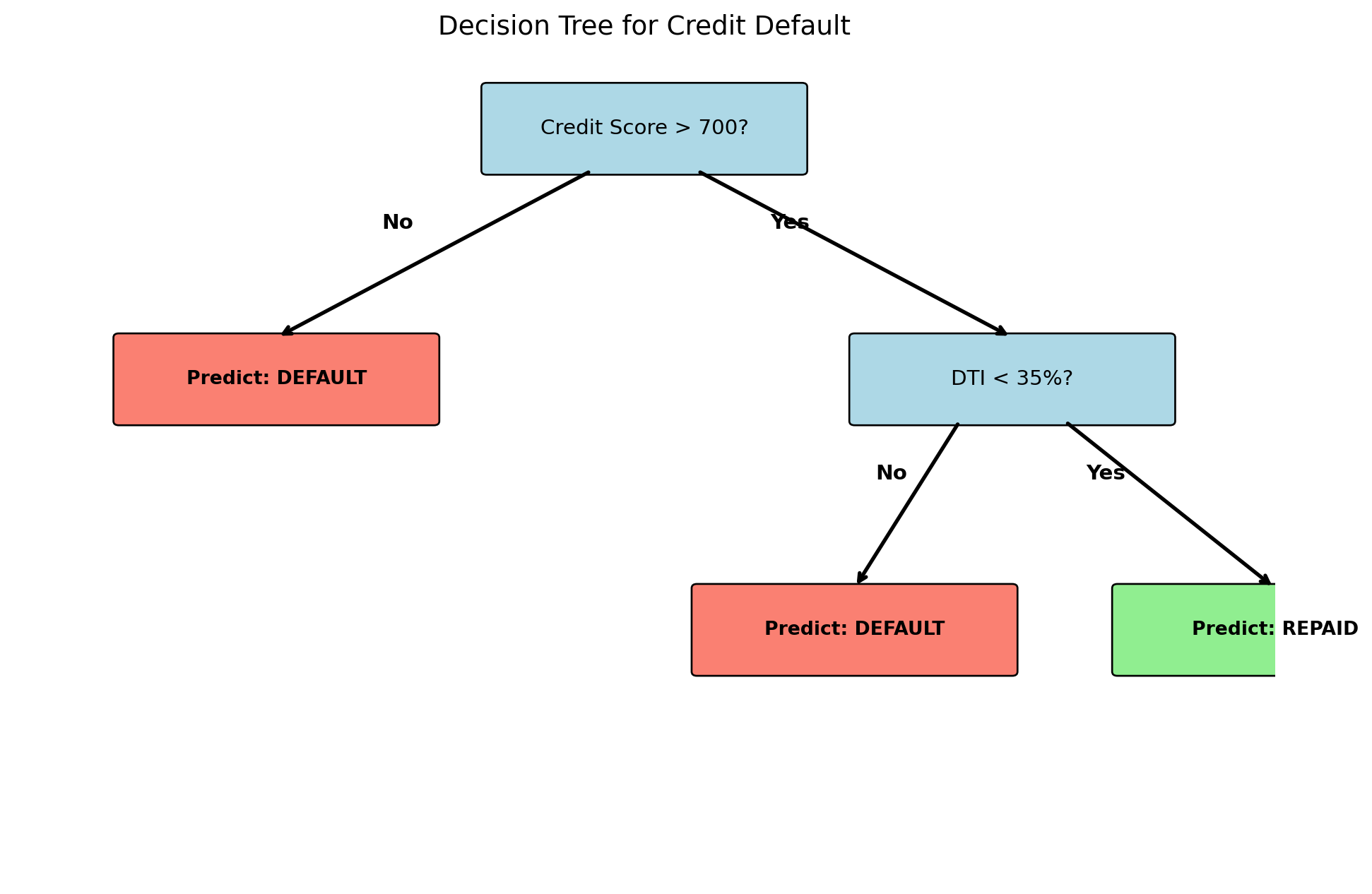
Decision trees mimic how humans make sequential decisions: a series of yes/no questions. Consider a loan officer evaluating an application. Is the credit score above 700? If no, deny. If yes, is the debt-to-income ratio below 35%? If no, deny. If yes, approve. Each question splits the applicant pool into subgroups, and predictions come from the subgroup an observation lands in.

Decision trees automate this process: they learn which questions (splits) to ask, on which features, and in what order. The result is a tree structure: the root node at the top asks the first question, internal nodes ask follow-up questions, and leaf nodes (or terminal nodes) at the bottom give predictions. Each path from root to leaf corresponds to a rule like “if credit score \(\geq\) 700 and DTI \(<\) 35%, predict repaid.”

6.2 Decision Trees as Partitions

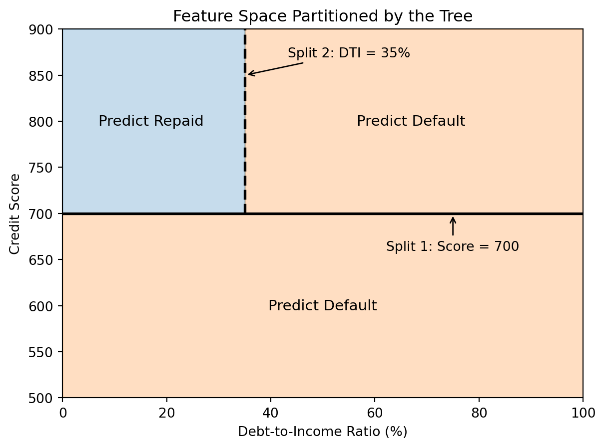
From a geometric perspective, each split divides the feature space with an axis-aligned line: “credit score \(= 700\)” is a horizontal line, “DTI \(= 35\%\)” is a vertical line. The tree recursively partitions the space into rectangular regions, and each region gets a single prediction.

6.3 How Trees Choose Splits

At every internal node, the tree needs to decide: which feature to split on, and at what value? The goal is to find the split that best separates the classes. A “pure” node (all one class) is ideal; a 50-50 mix is the worst.

Gini impurity measures how mixed a node is:

\[G = 1 - \sum_{k=1}^{K} \hat{p}_k^2\]

where \(\hat{p}_k\) is the proportion of observations in class \(k\). If a node contains only one class, \(G = 0\) (perfectly pure). If it’s a 50-50 mix of two classes, \(G = 0.5\) (maximum impurity). The tree tries every possible split on every feature and chooses the one that reduces impurity the most.

An alternative to Gini impurity is entropy:

\[H = -\sum_{k=1}^{K} \hat{p}_k \ln(\hat{p}_k)\]

Both measure the same thing — how mixed the classes are in a node — and usually produce similar trees. Gini impurity is the default in scikit-learn.

6.4 Fitting a Decision Tree

from sklearn.tree import DecisionTreeClassifier

# Generate credit data with two features
np.random.seed(123)
n = 500
credit_score = np.random.normal(700, 50, n)
dti = np.random.uniform(10, 50, n)

# Default probability depends on credit score and DTI
default_prob = 1 / (1 + np.exp(0.02 * (credit_score - 680) - 0.05 * (dti - 30)))
default_label = (np.random.random(n) < default_prob).astype(int)

X_tree = np.column_stack([credit_score, dti])
y_tree = default_label

# Fit a decision tree
tree = DecisionTreeClassifier(max_depth=3, random_state=42)
tree.fit(X_tree, y_tree);

print(f"Tree depth: {tree.get_depth()}")
print(f"Number of leaves: {tree.get_n_leaves()}")
print(f"Training accuracy: {tree.score(X_tree, y_tree):.3f}")

Tree depth: 3
Number of leaves: 8
Training accuracy: 0.704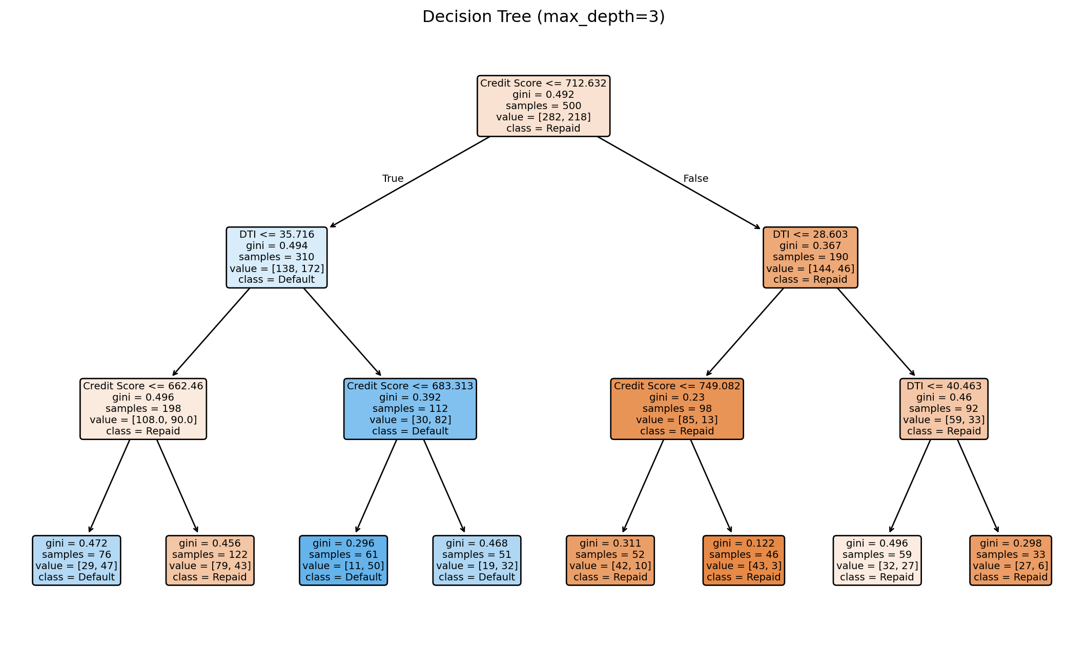

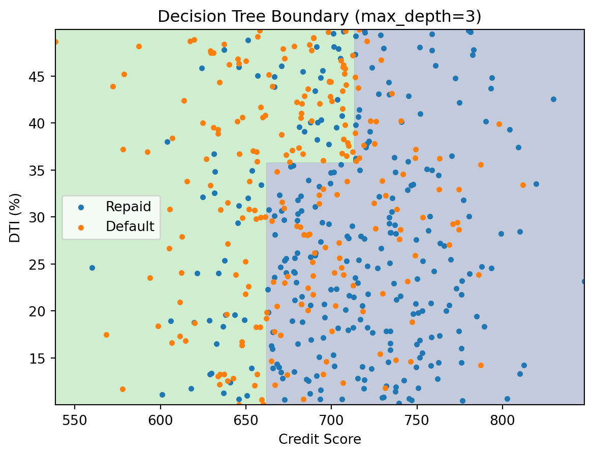
The decision boundary consists of axis-aligned rectangles. Each region gets a constant prediction — the majority class among the training points that land there.

6.5 Controlling Tree Complexity

An unrestricted decision tree can keep splitting until every leaf is pure (or every leaf contains a single point). This will achieve perfect accuracy on the training data, but it overfits badly — it memorizes the training noise and generalizes poorly.

We control complexity through hyperparameters:

max_depth: Maximum depth of the tree (how many levels of splits)
min_samples_split: Minimum number of samples required to split a node
min_samples_leaf: Minimum number of samples in each leaf

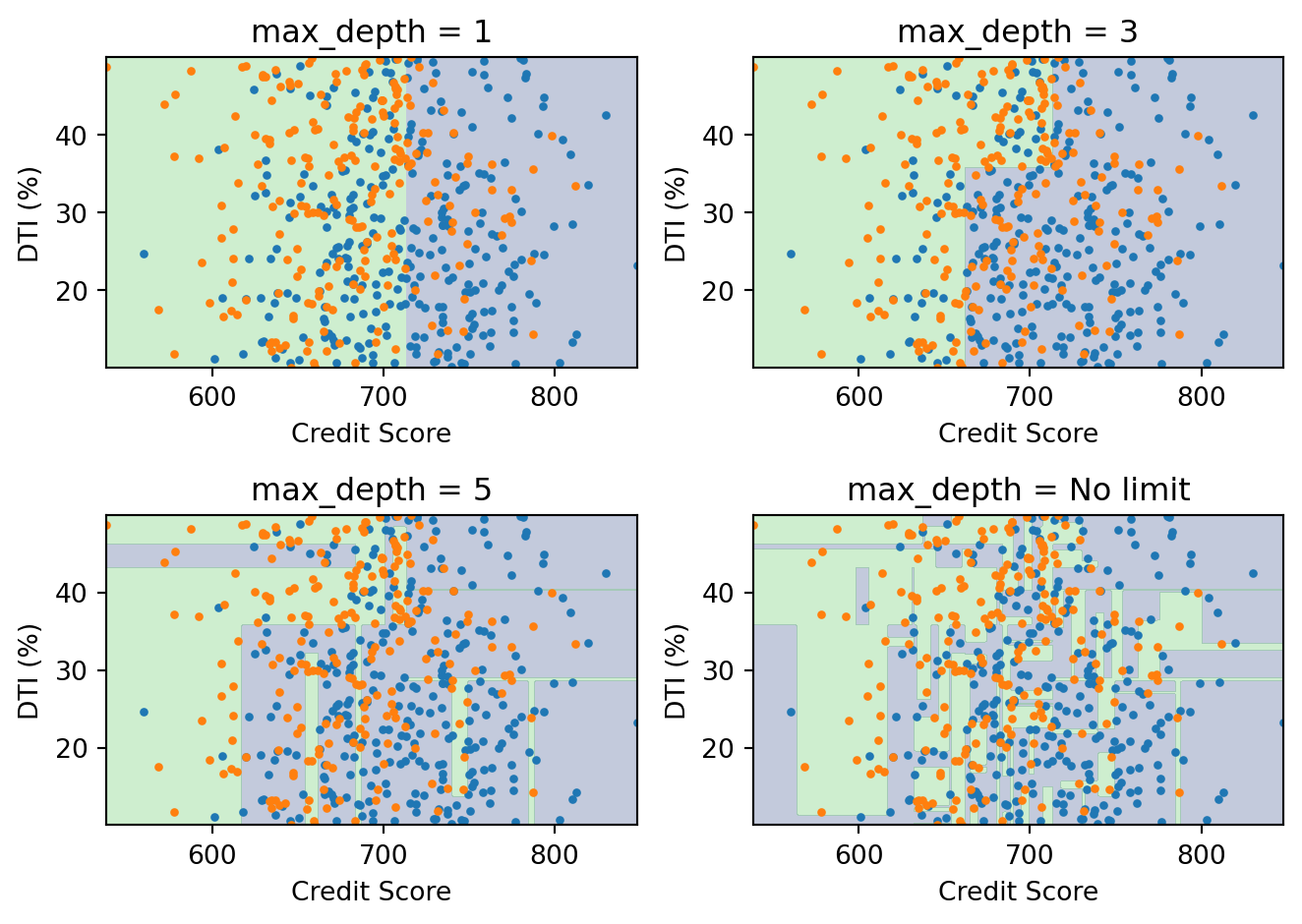
With max_depth=1, the tree makes a single split — too simple. With no depth limit, the boundary is jagged and overfits. A moderate depth (3–5) usually works best, and the exact value can be chosen by cross-validation.

We will revisit decision trees in the next lecture as the building block for ensemble methods (random forests and boosting), which address overfitting by combining many trees.

6.6 Strengths and Limitations

Decision trees are easy to interpret — you can trace any prediction through the tree and explain exactly why the model made that choice. They require no feature scaling, handle both numerical and categorical features, and naturally capture nonlinear relationships and interactions between features (a split on DTI within a branch that already split on credit score is an interaction).

The main limitation is instability: small changes in the training data can produce very different trees. A few observations shifting can change the first split, which cascades through the entire tree. This high variance is exactly what ensemble methods are designed to fix.

7 Evaluating Classification Models

7.1 Beyond Accuracy

In regression, we measured performance with MSE or \(R^2\). Classification needs different metrics because the outputs are discrete classes, not continuous values.

Accuracy — the fraction of correct predictions — is the most intuitive metric, but it can be misleading. Consider fraud detection where only 0.1% of transactions are fraudulent. A model that always predicts “not fraud” achieves 99.9% accuracy while catching zero fraud cases. Accuracy is useless when classes are imbalanced, which they almost always are in finance.

7.2 The Confusion Matrix

The confusion matrix is the foundation for all classification metrics. It’s a \(2 \times 2\) table that cross-tabulates actual classes against predicted classes:

	Predicted Negative	Predicted Positive
Actually Negative	True Negative (TN)	False Positive (FP)
Actually Positive	False Negative (FN)	True Positive (TP)

from sklearn.metrics import confusion_matrix

# Use logistic regression predictions on the default data
prob_pred = log_reg.predict_proba(X)[:, 1]
class_pred = (prob_pred > 0.5).astype(int)

cm = confusion_matrix(default, class_pred)
print("Confusion Matrix:")
print(cm)

Confusion Matrix:
[[961793   5207]
 [ 19202  13798]]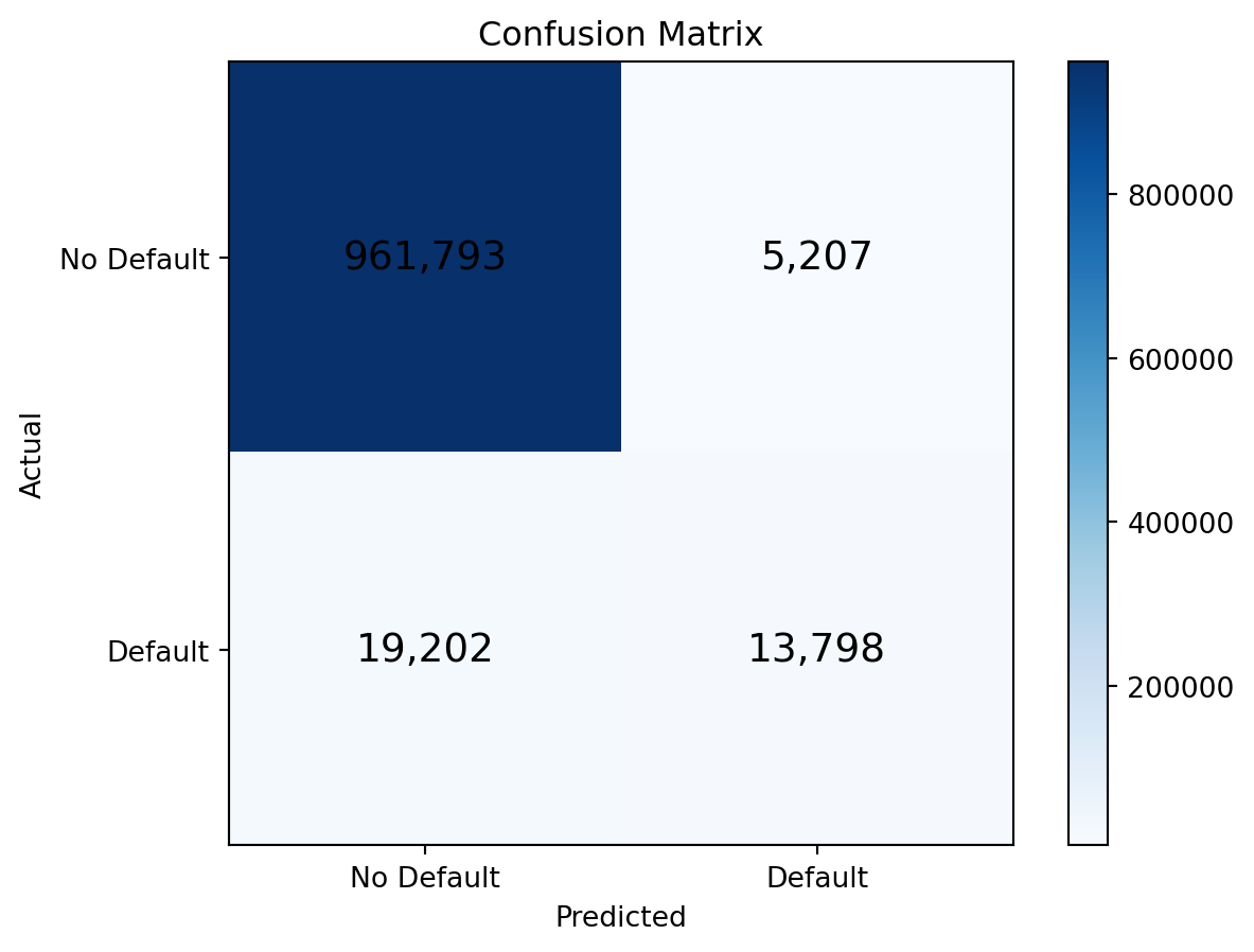

7.3 Precision and Recall

Two metrics derived from the confusion matrix are especially useful:

Precision answers: “of all the observations I predicted as positive, how many actually were?”

\[\text{Precision} = \frac{TP}{TP + FP}\]

Recall (also called sensitivity or true positive rate) answers: “of all the actually positive observations, how many did I catch?”

\[\text{Recall} = \frac{TP}{TP + FN}\]

from sklearn.metrics import precision_score, recall_score, f1_score

precision = precision_score(default, class_pred)
recall = recall_score(default, class_pred)
f1 = f1_score(default, class_pred)

print(f"Precision: {precision:.3f}")
print(f"Recall: {recall:.3f}")
print(f"F1 Score: {f1:.3f}")

Precision: 0.726
Recall: 0.418
F1 Score: 0.531

There is a fundamental tension between precision and recall. Lowering the threshold (predicting default more aggressively) catches more actual defaults (higher recall) but also flags more non-defaulters (lower precision). Raising the threshold does the opposite. The F1 score is one way to balance the two: it’s the harmonic mean of precision and recall, \(F_1 = 2 \cdot \frac{\text{Precision} \cdot \text{Recall}}{\text{Precision} + \text{Recall}}\).

In finance, the costs of false positives and false negatives are usually very different. Missing a default (false negative) costs the lender the full loan amount; flagging a good borrower (false positive) costs the lender the interest income. The right threshold depends on these costs, not on a mathematical formula.

7.4 The ROC Curve

The Receiver Operating Characteristic (ROC) curve shows how the tradeoff between true positive rate and false positive rate changes as we vary the classification threshold.

True Positive Rate (TPR) = Recall = \(\frac{TP}{TP + FN}\)
False Positive Rate (FPR) = \(\frac{FP}{FP + TN}\)

At threshold \(= 0\) we predict everything as positive: TPR \(= 1\) and FPR \(= 1\) (upper right). At threshold \(= 1\) we predict everything as negative: TPR \(= 0\) and FPR \(= 0\) (origin). The ROC curve traces the path between these two extremes as the threshold varies.

from sklearn.metrics import roc_curve, roc_auc_score

# Compute ROC curve
fpr, tpr, thresholds = roc_curve(default, prob_pred)
auc = roc_auc_score(default, prob_pred)

print(f"AUC: {auc:.4f}")

AUC: 0.9631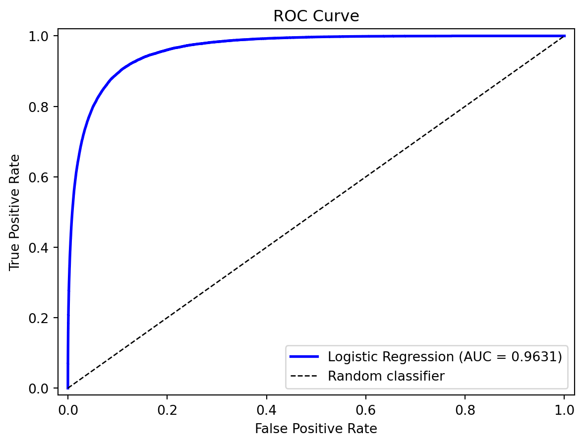

A perfect model hugs the upper-left corner (high TPR, low FPR). A random coin flip traces the diagonal. Any useful model should be above the diagonal.

7.5 AUC: Area Under the ROC Curve

The AUC (Area Under the ROC Curve) summarizes the ROC curve as a single number. It has a clean interpretation: the probability that the model ranks a randomly chosen positive observation higher than a randomly chosen negative observation.

AUC	Interpretation
1.0	Perfect classifier
0.9	Excellent
0.8	Good
0.7	Fair
0.5	Random guessing

AUC is threshold-independent — it evaluates the model’s ranking ability across all possible thresholds, not at any particular one. This makes it a good default metric for comparing models, especially when classes are imbalanced.

8 Summary

This chapter covered the core classification toolkit:

The linear probability model fails because it produces “probabilities” outside \([0, 1]\).
Logistic regression fixes this by wrapping a linear predictor in the sigmoid function. It’s a parametric, linear classifier: the decision boundary is a hyperplane. Coefficients have clean interpretations as log-odds. Regularization (lasso) controls overfitting.
LDA and QDA approach classification from a generative perspective, modelling what each class looks like and using Bayes’ theorem. LDA assumes shared covariance (linear boundary); QDA allows separate covariance (quadratic boundary).
Feature engineering can give logistic regression nonlinear boundaries, but requires knowing the right transformations in advance.
k-Nearest Neighbors classifies by majority vote of the \(k\) closest training points. It’s nonparametric and can learn any boundary shape, but struggles in high dimensions and requires careful choice of \(k\).
Decision trees recursively partition the feature space with axis-aligned splits, chosen to minimize impurity (Gini or entropy). They’re easy to interpret but prone to overfitting and instability — problems that ensemble methods (next lecture) are designed to fix.
Evaluation requires more than accuracy. The confusion matrix, precision, recall, and AUC provide different views of model performance. The right threshold depends on the relative costs of false positives and false negatives.

Appendix: Linear and Quadratic Discriminant Analysis

This appendix provides the full derivation of LDA and QDA. The main chapter introduced both methods briefly; here we work through the math in detail.

Why Another Classifier?

Logistic regression directly models \(P(y \,|\, \mathbf{x})\) — the probability of the class given the features. Discriminant analysis takes the opposite approach: model \(P(\mathbf{x} \,|\, y)\) — what the features look like within each class — and then use Bayes’ theorem to flip the conditioning.

This is the same distributional thinking from clustering (Lecture 4). In clustering, we assumed each group followed a distribution and tried to discover the groups. In discriminant analysis, we already know the groups and want to learn what makes them different. The table below makes the comparison explicit:

	Clustering (Lecture 4)	Logistic Regression	LDA
Type	Unsupervised	Supervised	Supervised
Labels	Unknown — discover them	Known — learn a boundary	Known — learn distributions
Strategy	Assume distributions; find groups	Directly model \(P(y \mid \mathbf{x})\)	Model \(P(\mathbf{x} \mid y)\) per class; apply Bayes

In practice, LDA and logistic regression often give similar answers. The value is in understanding both ways of thinking about classification.

Bayes’ Theorem for Classification

Suppose we have \(K\) classes labeled \(1, 2, \ldots, K\). Define:

\(\pi_k = P(y = k)\) — the prior probability of class \(k\) (how common is each class in the population?)
\(f_k(\mathbf{x}) = P(\mathbf{x} \,|\, y = k)\) — the likelihood (what do the features look like within class \(k\)?)

Bayes’ theorem gives us the posterior probability — the probability of class \(k\) given the observed features:

\[P(y = k \,|\, \mathbf{x}) = \frac{f_k(\mathbf{x}) \, \pi_k}{\sum_{j=1}^{K} f_j(\mathbf{x}) \, \pi_j}\]

The denominator is the same for all classes — it just ensures the posteriors sum to 1. We classify to the class with the highest posterior.

To use this formula, we need to specify \(f_k(\mathbf{x})\). LDA does this by assuming a multivariate normal distribution within each class.

The Normality Assumption

LDA assumes that within each class, the features follow a multivariate normal distribution with a class-specific mean but a shared covariance matrix:

\[\mathbf{x} \,|\, y = k \;\sim\; \mathcal{N}(\boldsymbol{\mu}_k, \boldsymbol{\Sigma})\]

The density function is:

\[f_k(\mathbf{x}) = \frac{1}{(2\pi)^{p/2} |\boldsymbol{\Sigma}|^{1/2}} \exp\left(-\frac{1}{2}(\mathbf{x} - \boldsymbol{\mu}_k)' \boldsymbol{\Sigma}^{-1}(\mathbf{x} - \boldsymbol{\mu}_k)\right)\]

where \(\boldsymbol{\mu}_k\) is the mean of class \(k\) (different for each class) and \(\boldsymbol{\Sigma}\) is the covariance matrix (same for all classes). Each class is a normal “blob” centred at \(\boldsymbol{\mu}_k\), but all classes share the same shape.

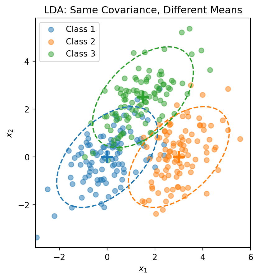
The dashed ellipses show the 95% probability contours — they have the same shape (orientation and spread) but different centres.

Deriving the Discriminant Function

We want to classify to the class with the highest posterior \(P(y = k \,|\, \mathbf{x})\). Taking the log:

\[\ln P(y = k \,|\, \mathbf{x}) = \ln f_k(\mathbf{x}) + \ln \pi_k - \underbrace{\ln \sum_{j} f_j(\mathbf{x}) \pi_j}_{\text{same for all } k}\]

Plugging in the normal density:

\[\ln f_k(\mathbf{x}) = -\frac{p}{2}\ln(2\pi) - \frac{1}{2}\ln|\boldsymbol{\Sigma}| - \frac{1}{2}(\mathbf{x} - \boldsymbol{\mu}_k)'\boldsymbol{\Sigma}^{-1}(\mathbf{x} - \boldsymbol{\mu}_k)\]

The first two terms don’t depend on \(k\) (because all classes share the same \(\boldsymbol{\Sigma}\)), so they cancel when comparing classes. Expanding the quadratic term:

\[(\mathbf{x} - \boldsymbol{\mu}_k)'\boldsymbol{\Sigma}^{-1}(\mathbf{x} - \boldsymbol{\mu}_k) = \mathbf{x}'\boldsymbol{\Sigma}^{-1}\mathbf{x} - 2\mathbf{x}'\boldsymbol{\Sigma}^{-1}\boldsymbol{\mu}_k + \boldsymbol{\mu}_k'\boldsymbol{\Sigma}^{-1}\boldsymbol{\mu}_k\]

The first piece, \(\mathbf{x}'\boldsymbol{\Sigma}^{-1}\mathbf{x}\), also doesn’t depend on \(k\). Dropping all terms that are constant across classes, we get the discriminant function:

\[\delta_k(\mathbf{x}) = \mathbf{x}' \boldsymbol{\Sigma}^{-1} \boldsymbol{\mu}_k - \frac{1}{2}\boldsymbol{\mu}_k' \boldsymbol{\Sigma}^{-1} \boldsymbol{\mu}_k + \ln \pi_k\]

This is a scalar — one number for each class \(k\). We classify \(\mathbf{x}\) to the class with the largest discriminant: \(\hat{y} = \arg\max_k \delta_k(\mathbf{x})\). The discriminant function is linear in \(\mathbf{x}\) — that’s why it’s called Linear Discriminant Analysis.

The Decision Boundary

The boundary between classes \(k\) and \(\ell\) is where \(\delta_k(\mathbf{x}) = \delta_\ell(\mathbf{x})\). Setting them equal and simplifying:

\[\mathbf{x}' \boldsymbol{\Sigma}^{-1} (\boldsymbol{\mu}_k - \boldsymbol{\mu}_\ell) = \frac{1}{2}(\boldsymbol{\mu}_k' \boldsymbol{\Sigma}^{-1} \boldsymbol{\mu}_k - \boldsymbol{\mu}_\ell' \boldsymbol{\Sigma}^{-1} \boldsymbol{\mu}_\ell) + \ln\frac{\pi_\ell}{\pi_k}\]

This is a linear equation in \(\mathbf{x}\), so the boundary is a line (in 2D) or hyperplane (in higher dimensions). With \(K\) classes there are \(K(K-1)/2\) pairwise boundaries, but only \(K - 1\) of them matter for defining the decision regions.

Estimating LDA Parameters

In practice, we estimate the parameters from training data:

Prior probabilities: \(\hat{\pi}_k = n_k / n\), where \(n_k\) is the number of training observations in class \(k\).

Class means: \(\hat{\boldsymbol{\mu}}_k = \frac{1}{n_k} \sum_{i:\, y_i = k} \mathbf{x}_i\)

Pooled covariance matrix:

\[\hat{\boldsymbol{\Sigma}} = \frac{1}{n - K} \sum_{k=1}^{K} \sum_{i:\, y_i = k} (\mathbf{x}_i - \hat{\boldsymbol{\mu}}_k)(\mathbf{x}_i - \hat{\boldsymbol{\mu}}_k)'\]

The pooled covariance averages the within-class covariances, weighted by class size. No optimization loop, no gradient descent — LDA computes its parameters in closed form from sample proportions, sample means, and the pooled covariance.

from sklearn.discriminant_analysis import LinearDiscriminantAnalysis

# Combine the 3-class data
X_lda = np.vstack([X1, X2, X3])
y_lda = np.array([0] * n_per_class + [1] * n_per_class + [2] * n_per_class)

# Fit LDA
lda = LinearDiscriminantAnalysis()
lda.fit(X_lda, y_lda)

print("LDA Class Means:")
for k in range(3):
    print(f"  Class {k}: {lda.means_[k]}")

print(f"\nClass Priors: {lda.priors_}")

LDA Class Means:
  Class 0: [ 0.00962094 -0.02608294]
  Class 1: [3.00835928 0.12294623]
  Class 2: [1.40152169 2.3715806 ]

Class Priors: [0.33333333 0.33333333 0.33333333]

# Visualize LDA decision boundaries
fig, ax = plt.subplots()

ax.scatter(X1[:, 0], X1[:, 1], alpha=0.5, label='Class 0')
ax.scatter(X2[:, 0], X2[:, 1], alpha=0.5, label='Class 1')
ax.scatter(X3[:, 0], X3[:, 1], alpha=0.5, label='Class 2')

# Decision boundaries
x_range = np.linspace(-3, 6, 200)
y_range = np.linspace(-3, 5, 200)
X_grid, Y_grid = np.meshgrid(x_range, y_range)
grid_points = np.column_stack([X_grid.ravel(), Y_grid.ravel()])
Z = lda.predict(grid_points).reshape(X_grid.shape)

ax.contour(X_grid, Y_grid, Z, levels=[0.5, 1.5], colors='black', linewidths=2)
ax.set_xlabel('$x_1$')
ax.set_ylabel('$x_2$')
ax.set_title('LDA Decision Boundaries')
ax.legend()
plt.show()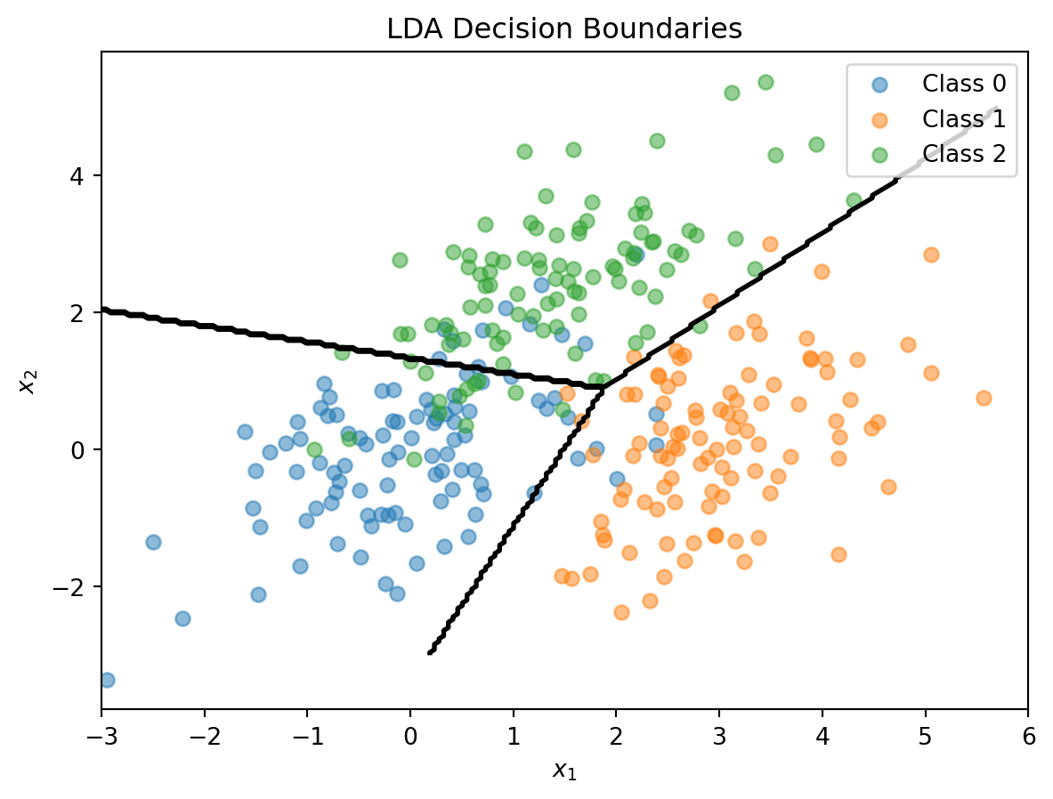

Quadratic Discriminant Analysis

LDA’s shared-covariance assumption is what makes the discriminant function linear in \(\mathbf{x}\). Quadratic Discriminant Analysis (QDA) relaxes this: each class gets its own covariance matrix \(\boldsymbol{\Sigma}_k\).

With separate covariances, the \(\mathbf{x}'\boldsymbol{\Sigma}^{-1}\mathbf{x}\) term no longer cancels (because \(\boldsymbol{\Sigma}_k^{-1}\) differs across classes), and the \(\ln|\boldsymbol{\Sigma}_k|\) term also varies. The discriminant function becomes:

\[\delta_k(\mathbf{x}) = -\frac{1}{2}\ln|\boldsymbol{\Sigma}_k| - \frac{1}{2}(\mathbf{x} - \boldsymbol{\mu}_k)' \boldsymbol{\Sigma}_k^{-1}(\mathbf{x} - \boldsymbol{\mu}_k) + \ln \pi_k\]

This is quadratic in \(\mathbf{x}\), giving curved decision boundaries.

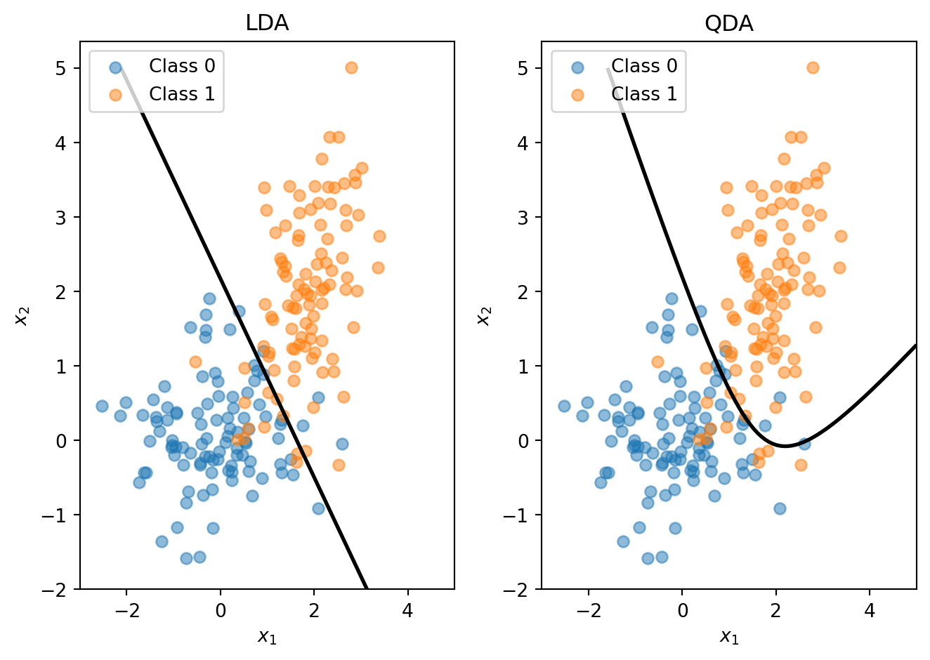
When classes genuinely have different covariances, QDA captures the curved boundary while LDA is forced to use a straight line.

The trade-off is straightforward:

LDA: More restrictive assumptions, fewer parameters, more stable with small samples
QDA: More flexible, more parameters, can overfit if sample size is small relative to the number of features

LDA and QDA both have good track records as classifiers, not necessarily because the normality assumption is correct, but because estimating fewer parameters (especially the shared \(\boldsymbol{\Sigma}\) in LDA) reduces variance. The decision boundary often works well even when normality is violated.

LDA vs. Logistic Regression

Both LDA and logistic regression produce linear decision boundaries. When should you use which?

Logistic regression makes no assumption about the distribution of \(\mathbf{x}\) — it models \(P(y \,|\, \mathbf{x})\) directly. This makes it more robust when the normality assumption is violated, and it’s preferred when features are binary or mixed types.

LDA is more efficient when normality actually holds, because it uses information about the class distributions. It can be more stable with small samples and naturally handles multi-class problems without any modification.

In practice, they often give similar results. Try both and compare via cross-validation.