Week 6: ML and Portfolio Theory

RSM338: Machine Learning in Finance

1 Introduction

Last week we studied regression and regularization — techniques for predicting continuous outcomes while controlling overfitting. This week we connect these tools to a core problem in finance: portfolio optimization.

1.1 The Complete Picture from RSM332

The challenge is familiar from RSM332: investors want to maximize return for a given level of risk. Harry Markowitz’s mean-variance framework, developed in the 1950s, provides the theoretical solution — work that earned him the Nobel Prize in Economics. The framework builds to an optimal portfolio in three steps.

Step 1: The Efficient Frontier. Given \(N\) risky assets, trace out the set of portfolios that offer the highest expected return for each level of risk. These are the “best available” combinations of risky assets.

Step 2: The Capital Allocation Line (CAL). Introduce a risk-free asset. The investor can now mix the risk-free asset with the tangency portfolio — the portfolio on the efficient frontier with the highest Sharpe ratio, where the CAL is tangent to the frontier. The CAL gives the best possible risk-return trade-off: a straight line from the risk-free rate through the tangency portfolio.

Step 3: Optimal Portfolio Choice. Where on the CAL does the investor land? That depends on preferences — their risk aversion \(\gamma\). A more risk-averse investor (\(\gamma\) high) holds more of the risk-free asset and less of the tangency portfolio. A less risk-averse investor (\(\gamma\) low) holds more risky assets, possibly leveraging.

This is the two-fund separation theorem: all investors hold the same risky portfolio (the tangency portfolio) combined with the risk-free asset. They differ only in the proportions.

The MVO solution \(\mathbf{w}^* = \frac{1}{\gamma}\boldsymbol{\Sigma}^{-1}\boldsymbol{\mu}\) encodes all three steps. The vector \(\boldsymbol{\Sigma}^{-1}\boldsymbol{\mu}\) gives the tangency portfolio weights — the same for every investor. The scalar \(\frac{1}{\gamma}\) just scales how much you invest in it versus the risk-free asset. Every optimal investor holds the same risky portfolio, just in different amounts — that’s why they all land on the same line (the CAL).

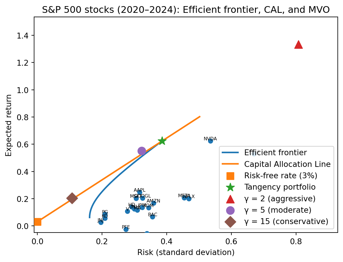
The plot below shows all three steps together using 20 S&P 500 stocks from 2020–2024: the efficient frontier traced from the data, the CAL through the tangency portfolio, and three MVO-optimal investors with different risk aversions landing at different points along the CAL.

The tangency portfolio (star) sits on the efficient frontier at the point of highest Sharpe ratio. The CAL runs from the risk-free rate through the tangency portfolio. The three MVO investors — aggressive (\(\gamma = 2\)), moderate (\(\gamma = 5\)), and conservative (\(\gamma = 15\)) — all land on the CAL, just at different points. The aggressive investor is further along the line (more invested in risky assets), while the conservative investor stays close to the risk-free rate.

1.2 Why Revisit Mean-Variance Optimization?

The MVO solution \(\mathbf{w}^* = \frac{1}{\gamma}\boldsymbol{\Sigma}^{-1}\boldsymbol{\mu}\) is elegant — but it has a hidden assumption: you need to know \(\boldsymbol{\mu}\) and \(\boldsymbol{\Sigma}\).

In practice, you must estimate them from data. Recall from Week 2 that plugging in estimates \(\hat{\mu}\) and \(\hat{\sigma}^2\) in place of the true parameters introduces estimation risk — additional uncertainty because our parameters are estimates, not truth. In Week 2, we saw this bias wealth forecasts upward. Here the consequences are worse: the MVO formula amplifies estimation error. Small errors in \(\hat{\boldsymbol{\mu}}\) and \(\hat{\boldsymbol{\Sigma}}\) get multiplied through the matrix inverse \(\boldsymbol{\Sigma}^{-1}\), producing wildly unstable portfolio weights.

This is the same “nearly singular inverse blows up” problem from Week 5 — but now it’s your money on the line.

1.3 The Gap Between Theory and Practice

In RSM332 (theory), \(\boldsymbol{\mu}\) and \(\boldsymbol{\Sigma}\) are known constants, the optimization formula gives the truly optimal portfolio, and more assets mean better diversification and higher utility. In practice, \(\boldsymbol{\mu}\) and \(\boldsymbol{\Sigma}\) must be estimated from noisy historical data, the “optimal” portfolio is optimal for the estimated parameters (not the true ones), and more assets mean more parameters to estimate, more estimation error, and often worse performance.

This is one of the biggest puzzles in applied finance: theoretically optimal portfolios often perform worse than naive strategies like equal weighting.

The rest of this chapter unpacks why. We start with the basics of mean-variance utility and the single-asset problem, build up to the multi-asset framework, quantify the cost of estimation error, and show how machine learning techniques — specifically Lasso regularization — can help close the gap between theory and practice.

2 Mean-Variance Utility

2.1 The Investor’s Problem

An investor must decide how to allocate wealth between assets with different risk and return characteristics. This is one of the most fundamental problems in finance. But before we can solve it, we need a framework for comparing portfolios. How do we rank a portfolio with 12% expected return and 20% volatility against one with 8% expected return and 12% volatility? We need a way to balance the competing objectives of seeking higher returns while avoiding excessive risk.

From RSM332, you know that most investors are risk-averse—they prefer certainty to uncertainty. Given two investments with the same expected return, a risk-averse investor chooses the less risky one every time. Conversely, to accept more risk, they demand higher expected return as compensation. This trade-off between risk and return is at the heart of investment decisions.

Risk aversion isn’t irrational—it reflects the diminishing marginal utility of wealth. An extra $10,000 means more to you when you have $50,000 than when you have $5,000,000. Because losses hurt more than gains feel good (relative to your current wealth), investors rationally avoid unnecessary uncertainty even if it doesn’t change their expected outcome.

2.2 The Utility Function

To formalize how investors rank portfolios, we assume they use a utility function—a formula that assigns a number to each portfolio representing how “good” it is to the investor. Higher utility means a better portfolio. The investor’s goal is then simple: choose the portfolio with the highest utility.

For a portfolio with return \(r_p\), we define:

• \(\mu_p = \mathbb{E}[r_p]\): the expected return of the portfolio
• \(\sigma_p^2 = \text{Var}(r_p)\): the variance (our measure of risk)

The notation uses Greek letters that are standard in finance and statistics: \(\mu\) (mu) for expected values and \(\sigma\) (sigma) for standard deviation. The squared term \(\sigma^2\) is the variance.

The mean-variance utility function captures the trade-off between return and risk in a simple formula: \[U(r_p) = \mu_p - \frac{\gamma}{2} \sigma_p^2\]

Let’s unpack each component:

• \(\mu_p\) is expected return—investors want this to be high
• \(\sigma_p^2\) is variance—investors want this to be low
• \(\gamma\) (gamma) is the risk aversion parameter—how much the investor penalizes risk
• The \(\frac{1}{2}\) is a mathematical convenience that makes derivatives work out cleanly

In words: utility equals expected return minus a penalty for risk. The penalty is proportional to variance, and the risk aversion parameter \(\gamma\) determines how severe that penalty is. More risk-averse investors have higher \(\gamma\) and penalize variance more heavily.

Why this specific functional form? It emerges naturally from assuming that investors have quadratic utility over final wealth, or equivalently that returns are normally distributed and investors have exponential utility. These assumptions are imperfect—real returns have fat tails, and real preferences may be more complex—but mean-variance utility captures the essential trade-off and is tractable enough to optimize analytically.

2.3 Risk Aversion

The parameter \(\gamma\) quantifies the investor’s attitude toward risk:

• \(\gamma = 0\): Risk neutral. The investor cares only about expected return, completely ignoring risk. They would accept any gamble with positive expected value, no matter how risky.
• \(\gamma > 0\): Risk averse. The investor demands compensation for bearing risk. This is the typical, empirically realistic case.
• \(\gamma < 0\): Risk seeking. The investor actually enjoys taking risk. While unusual, some behaviors (like buying lottery tickets) suggest risk-seeking in certain domains.

Empirical estimates suggest typical investors have \(\gamma\) between 2 and 10, though this varies widely across individuals and circumstances. With \(\gamma = 2\), accepting 1 percentage point more variance requires roughly 1 percentage point more expected return to maintain the same utility. With \(\gamma = 10\), the same increase in variance would require 5 percentage points more expected return—this investor is much more conservative.

To see how \(\gamma\) affects choices concretely: suppose a portfolio has 10% expected return and 20% standard deviation (so 4% variance). With \(\gamma = 2\), the utility is \(0.10 - \frac{2}{2} \times 0.04 = 0.10 - 0.04 = 0.06\). With \(\gamma = 10\), the utility is \(0.10 - \frac{10}{2} \times 0.04 = 0.10 - 0.20 = -0.10\). The more risk-averse investor views this risky portfolio as worse than holding cash!

2.4 Certainty Equivalent

The mean-variance utility has a nice interpretation as the certainty equivalent—the guaranteed (risk-free) return that would make the investor indifferent between holding the risky portfolio or receiving the guarantee.

If a portfolio has utility \(U(r_p) = 0.05\), this means the investor views it as equivalent to a guaranteed 5% return. They would be equally happy receiving 5% for sure or holding the risky portfolio. The certainty equivalent is always below the expected return for a risk-averse investor—they’re willing to accept a lower guaranteed return to avoid uncertainty.

Consider a portfolio with 12% expected return and 20% standard deviation. For an investor with \(\gamma = 2\): \[U = 0.12 - \frac{2}{2} \times (0.20)^2 = 0.12 - 0.04 = 0.08\]

This investor views the risky 12% expected return portfolio as equivalent to a guaranteed 8% return. The 4 percentage point gap is the “price” they implicitly pay for the uncertainty—the risk premium they’d forgo to eliminate the risk.

3 Optimal Portfolio: Single Risky Asset

3.1 Setting Up the Problem

Consider the simplest possible portfolio problem: one risky asset (say, a stock index like the S&P 500) and a risk-free asset (T-bills or government bonds). The investor must decide what fraction of their wealth to put in stocks versus bonds.

Let \(w\) be the fraction of wealth invested in the risky asset. Then \(1-w\) goes to the risk-free asset. There’s no constraint that \(w\) be between 0 and 1—if \(w > 1\), the investor is borrowing at the risk-free rate to lever up their stock position; if \(w < 0\), they’re shorting the risky asset.

We work with excess returns—returns above the risk-free rate: \[r_t = R_t - R_f\]

where \(R_t\) is the total return on the risky asset and \(R_f\) is the risk-free rate. Why excess returns? It simplifies the math considerably. When you hold \(w\) in the risky asset and \(1-w\) in the risk-free asset, your total return is \(w \cdot R_t + (1-w) \cdot R_f = R_f + w(R_t - R_f) = R_f + w \cdot r_t\). The excess return of your portfolio is just \(w \cdot r_t\)—the risk-free portion contributes nothing to excess return. This means we can ignore the risk-free asset entirely when optimizing over \(w\).

3.2 Portfolio Mean and Variance

Since the portfolio’s excess return is simply \(r_{p,t} = w \cdot r_t\), we can easily compute its mean and variance using the scaling properties from Week 1.

Expected excess return: \[\mu_p = \mathbb{E}[w \cdot r_t] = w \cdot \mathbb{E}[r_t] = w \cdot \mu\]

The expected return scales linearly with the weight. If you double your stock position, you double your expected excess return.

Variance: \[\sigma_p^2 = \text{Var}(w \cdot r_t) = w^2 \cdot \text{Var}(r_t) = w^2 \cdot \sigma^2\]

Variance scales with the square of the weight. This is because variance measures squared deviations from the mean.

Standard deviation: \[\sigma_p = |w| \cdot \sigma\]

Here \(\mu\) and \(\sigma^2\) are the expected excess return and variance of the risky asset. The absolute value appears because standard deviation is always positive, but \(w\) could be negative (if shorting).

3.3 The Sharpe Ratio

When \(w > 0\) (positive investment in the risky asset), notice something remarkable: \[\frac{\mu_p}{\sigma_p} = \frac{w \cdot \mu}{w \cdot \sigma} = \frac{\mu}{\sigma}\]

The ratio of expected return to standard deviation is constant, regardless of how much you invest! The \(w\)’s cancel out.

This ratio \(\frac{\mu}{\sigma}\) is the Sharpe ratio of the risky asset, named after Nobel laureate William Sharpe. From RSM332, you may recall that the Sharpe ratio measures reward per unit of risk—how much expected return you get for each unit of volatility you bear.

The Sharpe ratio being constant means that by adjusting \(w\), you can move along a straight line in risk-return space. You can take more or less risk, but you can’t improve the Sharpe ratio—it’s determined by the risky asset itself. All you can do is decide where along the line to position yourself.

This geometric insight is central to mean-variance theory: with one risky asset and a risk-free asset, all efficient portfolios lie on a line (the Capital Allocation Line), and the slope of that line is the Sharpe ratio.

3.4 Finding the Optimal Weight

The investor’s problem is to choose \(w\) to maximize utility. Substituting the portfolio mean and variance into the utility function: \[U(w) = w\mu - \frac{\gamma}{2} w^2 \sigma^2\]

This is a quadratic function of \(w\). The coefficient on \(w^2\) is \(-\frac{\gamma}{2}\sigma^2\), which is negative (since \(\gamma > 0\) and \(\sigma^2 > 0\)). When a quadratic opens downward, it has a unique maximum at its vertex.

To find the maximum, we take the derivative with respect to \(w\) and set it equal to zero. The derivative of \(w\mu\) is \(\mu\), and the derivative of \(-\frac{\gamma}{2}w^2\sigma^2\) is \(-\gamma w \sigma^2\): \[\frac{dU}{dw} = \mu - \gamma w \sigma^2 = 0\]

Solving for \(w\): \[\gamma w \sigma^2 = \mu\] \[w^* = \frac{1}{\gamma} \cdot \frac{\mu}{\sigma^2}\]

This elegant formula tells us exactly how much to invest in the risky asset.

3.5 Interpreting the Formula

The optimal weight formula \(w^* = \frac{\mu}{\gamma \sigma^2}\) decomposes into interpretable pieces:

• \(\frac{1}{\gamma}\): Less risk-averse investors (smaller \(\gamma\)) invest more in the risky asset. If you’re comfortable with risk, you take more of it.
• \(\mu\): Higher expected return → invest more. This is intuitive—better opportunities deserve larger positions.
• \(\frac{1}{\sigma^2}\): Higher variance → invest less. Riskier assets get smaller allocations.

The ratio \(\frac{\mu}{\sigma^2}\) is sometimes called the reward-to-variance ratio. It differs from the Sharpe ratio (\(\frac{\mu}{\sigma}\)) by having variance instead of standard deviation in the denominator.

Example: Suppose the risky asset has expected excess return \(\mu = 8\%\) per year and standard deviation \(\sigma = 20\%\) (so variance \(\sigma^2 = 0.04\)).

For a moderately risk-averse investor with \(\gamma = 2\): \[w^* = \frac{0.08}{2 \times 0.04} = \frac{0.08}{0.08} = 1.0\]

This investor puts 100% of wealth in the risky asset, nothing in T-bills.

For a more risk-averse investor with \(\gamma = 4\): \[w^* = \frac{0.08}{4 \times 0.04} = \frac{0.08}{0.16} = 0.5\]

This investor puts 50% in stocks and 50% in T-bills—a more conservative allocation.

For a very risk-averse investor with \(\gamma = 10\): \[w^* = \frac{0.08}{10 \times 0.04} = \frac{0.08}{0.40} = 0.2\]

Only 20% goes to stocks. The rest sits safely in T-bills.

3.6 Achieved Utility

What utility does the investor achieve at the optimal weight? We can substitute \(w^* = \frac{\mu}{\gamma \sigma^2}\) back into the utility function:

\[\begin{align*} U(w^*) &= w^* \mu - \frac{\gamma}{2} (w^*)^2 \sigma^2 \\ &= \frac{\mu}{\gamma \sigma^2} \cdot \mu - \frac{\gamma}{2} \cdot \frac{\mu^2}{\gamma^2 \sigma^4} \cdot \sigma^2 \\ &= \frac{\mu^2}{\gamma \sigma^2} - \frac{\mu^2}{2\gamma \sigma^2} \\ &= \frac{\mu^2}{2\gamma \sigma^2} \end{align*}\]

We can write this more compactly using the Sharpe ratio \(\theta = \frac{\mu}{\sigma}\): \[U(w^*) = \frac{\theta^2}{2\gamma}\]

This formula reveals that optimal utility depends on the squared Sharpe ratio. A risky asset with twice the Sharpe ratio delivers four times the utility (for a given risk aversion). Better risk-adjusted returns translate directly into higher achievable welfare.

4 The Estimation Problem

4.1 From Theory to Practice

The optimal weight formula is elegant and intuitive: \[w^* = \frac{\mu}{\gamma \sigma^2}\]

But there’s a fundamental problem: we don’t know \(\mu\) and \(\sigma^2\).

These are “population” parameters—the true values from the underlying probability distribution of returns. They represent what we’d observe if we could see infinitely many draws from the distribution. But we can’t. We only have historical data: a finite sample of past returns.

In practice, we must estimate these parameters from the data. Estimates are denoted with “hats” to distinguish them from the true values:

• \(\hat{\mu}\): the estimated expected return (computed from historical data)
• \(\hat{\sigma}^2\): the estimated variance

The hat notation is a reminder that these are approximations, not the truth. And as we’ll see, the gap between estimate and truth can be substantial.

4.2 Estimating Expected Return

Given \(T\) historical excess returns \(r_1, r_2, \ldots, r_T\), the natural estimate of expected return is the sample mean: \[\hat{\mu} = \frac{1}{T} \sum_{t=1}^{T} r_t\]

In words: average the historical returns. This is the estimator you’d naturally think of, and it has good statistical properties. It’s unbiased—on average, across many samples, it equals the true \(\mu\). Mathematically, \(\mathbb{E}[\hat{\mu}] = \mu\).

But “unbiased” doesn’t mean “accurate.” Any particular estimate \(\hat{\mu}\) differs from the true \(\mu\) due to randomness in the sample. If you had drawn a different sample (observed a different historical period), you’d get a different \(\hat{\mu}\). This variability is estimation risk—the uncertainty inherent in using sample statistics to infer population parameters.

4.3 How Precise Is the Estimate?

Just how uncertain is our estimate? Let’s quantify it with a confidence interval using real data.

With US stock market data from 1926-2023 (about 98 years), suppose we find \(\hat{\mu} = 8.52\%\) and \(\hat{\sigma} = 20.19\%\). How confident can we be that the true \(\mu\) is close to 8.52%?

The standard error of the sample mean is: \[SE(\hat{\mu}) = \frac{\sigma}{\sqrt{T}} \approx \frac{0.2019}{\sqrt{98}} \approx 0.0204\]

A 95% confidence interval is approximately: \[\mu \in \hat{\mu} \pm 1.96 \times SE \approx 8.52\% \pm 4.0\%\]

So the 95% confidence interval is roughly \((4.5\%, 12.5\%)\).

Even with nearly a century of data, we can’t pin down whether the true expected return is 4.5% or 12.5%! This is an enormous range. The difference between 4.5% and 12.5% expected return is the difference between “stocks barely beat bonds” and “stocks are a fantastic investment.” Yet the data don’t distinguish between these very different worlds.

4.4 Why Is Expected Return So Hard to Estimate?

The precision of our estimate depends on two factors:

1. Sample size (\(T\)): More data helps, but the improvement is slow. The standard error decreases as \(\frac{1}{\sqrt{T}}\). To cut uncertainty in half, you need four times as much data. To get from 98 years to half the uncertainty, you’d need 392 years!

2. Volatility (\(\sigma\)): Higher volatility means more noise obscuring the signal. The standard error is proportional to \(\sigma\).

For stocks, the signal-to-noise ratio is terrible. With annual data:

• Expected excess return (signal): ~8%
• Standard deviation (noise): ~20%

The signal is tiny compared to the noise. Each year, the stock market bounces around by roughly 20%, but the underlying expected return we’re trying to estimate is only 8%. It’s like trying to measure a 8-inch object with a ruler that has 20-inch random errors.

This is why Goyal and Welch (2008) found that most return predictors fail out-of-sample—expected returns are simply very hard to estimate reliably. Variables that seem to predict returns in historical data often fail when applied to new data, because the apparent predictive power was just fitting noise.

4.5 Uncertainty Propagates to Weights

If we use \(\hat{\mu}\) in the optimal weight formula: \[\hat{w} = \frac{\hat{\mu}}{\gamma \sigma^2}\]

(assuming \(\sigma^2\) is known for now, to isolate the effect of estimating \(\mu\))

The randomness in \(\hat{\mu}\) flows directly into \(\hat{w}\). Since \(\hat{w}\) is just a scaled version of \(\hat{\mu}\), the uncertainty scales too.

Under the assumption that returns are i.i.d. normal, the sample mean has a normal distribution: \[\hat{\mu} \sim N\left(\mu, \frac{\sigma^2}{T}\right)\]

Since \(\hat{w} = \frac{\hat{\mu}}{\gamma \sigma^2}\), it’s also normally distributed: \[\hat{w} \sim N\left(w^*, \frac{1}{T \gamma^2 \sigma^2}\right)\]

where \(w^* = \frac{\mu}{\gamma \sigma^2}\) is the true optimal weight.

From our confidence interval \(\mu \in (4.5\%, 12.5\%)\), with \(\gamma = 2\) and \(\sigma^2 = 0.04\), the implied range for \(w^*\) is: \[w^* \in \left(\frac{0.045}{2 \times 0.04}, \frac{0.125}{2 \times 0.04}\right) = (0.56, 1.56)\]

This is a huge range for such a basic investment decision. At one end, the investor should put 56% in stocks; at the other end, 156% (levered!). The data don’t tell us which is right.

5 Utility Loss from Estimation

5.1 The Cost of Estimated Weights

When we use the estimated weight \(\hat{w}\) instead of the true optimal \(w^*\), we achieve lower utility. This is inevitable: \(w^*\) is optimal by definition, so any deviation from it—including deviations caused by estimation error—reduces utility.

To quantify this loss, we compute the expected utility when using estimated weights. The expectation is over the randomness in estimation—different samples give different \(\hat{\mu}\), hence different \(\hat{w}\).

The utility from using \(\hat{w}\), evaluated at the true parameters \(\mu\) and \(\sigma^2\), is: \[U(\hat{w}) = \hat{w} \mu - \frac{\gamma}{2} \hat{w}^2 \sigma^2\]

Taking expectations over the sampling distribution of \(\hat{w}\): \[\mathbb{E}[U(\hat{w})] = \mathbb{E}[\hat{w}] \mu - \frac{\gamma}{2} \mathbb{E}[\hat{w}^2] \sigma^2\]

Since \(\hat{w}\) is unbiased, \(\mathbb{E}[\hat{w}] = w^*\). For the second moment, we use \(\mathbb{E}[\hat{w}^2] = (w^*)^2 + \text{Var}(\hat{w}) = (w^*)^2 + \frac{1}{T\gamma^2\sigma^2}\).

After working through the algebra: \[\mathbb{E}[U(\hat{w})] = U(w^*) - \frac{1}{2T\gamma}\]

5.2 Understanding the Utility Loss

The expected utility loss from estimation is: \[\text{Utility Loss} = U(w^*) - \mathbb{E}[U(\hat{w})] = \frac{1}{2T\gamma}\]

This formula is revealing:

• More data (\(T\) larger) helps: The loss decreases as \(\frac{1}{T}\). With more historical returns, our estimates improve, and we get closer to the true optimum.
• More risk-averse investors lose less: Higher \(\gamma\) means smaller positions in the risky asset. Smaller positions are less exposed to estimation error—if you’re barely invested, it matters less whether your estimate is wrong.

Let’s make this concrete. With \(T = 10\) years of annual data and \(\gamma = 2\): \[\text{Utility Loss} = \frac{1}{2 \times 10 \times 2} = 0.025\]

This is 2.5 percentage points of certainty-equivalent return lost to estimation error every year. If the true optimal utility is 8% (the certainty equivalent of the optimal portfolio), using estimated weights gives only 5.5% expected utility. That’s a substantial cost.

With monthly data (\(T = 120\)), the loss drops to \(\frac{1}{2 \times 120 \times 2} = 0.002\)—just 0.2 percentage points. More data helps considerably.

5.3 The Reality Is Even Worse

Our analysis assumed \(\sigma^2\) was known, isolating the effect of estimating \(\mu\). In practice, we estimate variance too:

\[\hat{\sigma}^2 = \frac{1}{T-1} \sum_{t=1}^{T} (r_t - \hat{\mu})^2\]

With both \(\hat{\mu}\) and \(\hat{\sigma}^2\) estimated, the utility loss is larger than \(\frac{1}{2T\gamma}\). The exact formula is more complex, but the intuition is the same: using estimated parameters instead of true parameters costs utility, the loss decreases with more data (but slowly), and short samples — typical in finance — lead to substantial estimation risk.

5.4 Multiple Assets Make It Worse

With \(N\) risky assets instead of just one, the utility loss becomes: \[\text{Utility Loss} = \frac{N}{2\gamma T}\]

The loss is proportional to \(N\), the number of assets! This is bad news for diversification.

Why does adding assets make estimation worse? With more assets:

• More expected returns to estimate (one \(\mu_i\) for each asset)
• Each estimate has error
• The optimizer uses all these noisy estimates simultaneously
• Errors compound and interact in the optimization

This is the curse of dimensionality in portfolio optimization. More assets theoretically offer better diversification—more opportunities to reduce risk. But more assets also mean more parameters to estimate, and with limited data, more parameters mean more estimation error.

Example: Consider \(N = 25\) assets (a typical industry portfolio), \(T = 60\) months (5 years of monthly data), and \(\gamma = 2\): \[\text{Utility Loss} = \frac{25}{2 \times 2 \times 60} = \frac{25}{240} = 0.104\]

That’s a loss of 10.4 percentage points of certainty equivalent! If the true optimal utility is 15% (reflecting the gains from diversification), the expected utility with estimated weights is only: \[\mathbb{E}[U(\hat{\mathbf{w}})] = 0.15 - 0.104 = 0.046\]

Estimation error wipes out two-thirds of the benefit of optimization. The diversification that theory promises is largely eaten up by estimation error in practice.

6 The Mean-Variance Frontier

6.1 Multiple Assets: Vector Notation

With \(N\) risky assets, we need vectors and matrices to express the portfolio problem. This notation is standard in finance and lets us state the multi-asset problem compactly.

• \(\mathbf{r}_t\): the \(N \times 1\) vector of excess returns at time \(t\). Each element \(r_{i,t}\) is the excess return of asset \(i\).
• \(\boldsymbol{\mu}\): the \(N \times 1\) vector of expected excess returns. The \(i\)-th element is \(\mu_i = \mathbb{E}[r_i]\).
• \(\boldsymbol{\Sigma}\): the \(N \times N\) covariance matrix. The diagonal elements are variances: \(\Sigma_{ii} = \text{Var}(r_i)\). The off-diagonal elements are covariances: \(\Sigma_{ij} = \text{Cov}(r_i, r_j)\) for \(i \neq j\).
• \(\mathbf{w}\): the \(N \times 1\) vector of portfolio weights on risky assets only. The \(i\)-th element \(w_i\) is the fraction invested in asset \(i\). We don’t require \(\mathbf{w}^\prime \mathbf{1} = 1\) — the remainder \(1 - \mathbf{w}^\prime \mathbf{1}\) is invested in the risk-free asset.

The covariance matrix captures all the variance and covariance information in a single object. It’s always symmetric (\(\Sigma_{ij} = \Sigma_{ji}\)) and positive semi-definite (portfolio variance can’t be negative).

Portfolio expected excess return: \[\mu_p = \mathbf{w}^\prime \boldsymbol{\mu} = \sum_{i=1}^{N} w_i \mu_i\]

The prime notation (\(^\prime\)) denotes transpose. This is a weighted average of individual expected excess returns.

Portfolio variance: \[\sigma_p^2 = \mathbf{w}^\prime \boldsymbol{\Sigma} \mathbf{w} = \sum_{i=1}^{N} \sum_{j=1}^{N} w_i w_j \Sigma_{ij}\]

This expression shows that portfolio variance depends on all the variances AND all the covariances. When assets are positively correlated, the covariance terms add to portfolio risk; when they’re negatively correlated, they reduce it. This is the mathematical basis for diversification.

6.2 The Optimal Portfolio (Multiple Assets)

The investor maximizes utility: \[U(\mathbf{w}) = \mathbf{w}^\prime \boldsymbol{\mu} - \frac{\gamma}{2} \mathbf{w}^\prime \boldsymbol{\Sigma} \mathbf{w}\]

Taking derivatives and setting equal to zero (using vector calculus): \[\frac{\partial U}{\partial \mathbf{w}} = \boldsymbol{\mu} - \gamma \boldsymbol{\Sigma} \mathbf{w} = \mathbf{0}\]

Solving for \(\mathbf{w}\): \[\gamma \boldsymbol{\Sigma} \mathbf{w} = \boldsymbol{\mu}\] \[\mathbf{w}^* = \frac{1}{\gamma} \boldsymbol{\Sigma}^{-1} \boldsymbol{\mu}\]

This is the multi-asset analog of \(w^* = \frac{\mu}{\gamma \sigma^2}\). The covariance matrix \(\boldsymbol{\Sigma}\) generalizes \(\sigma^2\), and we need its inverse \(\boldsymbol{\Sigma}^{-1}\). Inverting a matrix is the multivariate equivalent of dividing by variance.

The matrix \(\boldsymbol{\Sigma}^{-1}\) does sophisticated work:

• It adjusts for different volatilities—more volatile assets get lower weights, all else equal
• It accounts for correlations—when two assets are highly correlated, holding both is partially redundant, so the inverse matrix implicitly reduces positions in redundant assets
• It enables diversification—assets with low correlations to others get higher weights because they provide unique diversification benefits

The optimal portfolio utility becomes: \[U(\mathbf{w}^*) = \frac{\theta^2}{2\gamma}, \quad \text{where} \quad \theta^2 = \boldsymbol{\mu}^\prime \boldsymbol{\Sigma}^{-1} \boldsymbol{\mu}\]

Here \(\theta\) is the Sharpe ratio of the optimal (tangency) portfolio—the best possible risk-adjusted return achievable from the \(N\) assets.

6.3 The Power of Diversification

The correlation between assets determines how much diversification helps. To see this, consider two assets — bonds (6% expected return, 12% volatility) and stocks (12% expected return, 22% volatility) — and vary the correlation between them.

import numpy as np
import matplotlib.pyplot as plt

# Two assets
mu_A, sigma_A = 0.06, 0.12  # Bonds
mu_B, sigma_B = 0.12, 0.22  # Stocks

# Different correlations
correlations = [1.0, 0.3, -0.5, -1.0]

fig, ax = plt.subplots()

for rho in correlations:
    weights = np.linspace(0, 1, 100)
    mus_plot = []
    sigmas_plot = []

    for w in weights:
        mu_p = w * mu_B + (1 - w) * mu_A
        var_p = (w * sigma_B)**2 + ((1-w) * sigma_A)**2 + 2*w*(1-w)*rho*sigma_A*sigma_B
        mus_plot.append(mu_p)
        sigmas_plot.append(np.sqrt(max(var_p, 0)))

    ax.plot(sigmas_plot, mus_plot, label=f'ρ = {rho}')

ax.scatter([sigma_A], [mu_A], s=100, zorder=5)
ax.scatter([sigma_B], [mu_B], s=100, zorder=5)
ax.annotate('Bonds', (sigma_A, mu_A), textcoords="offset points", xytext=(10,-10))
ax.annotate('Stocks', (sigma_B, mu_B), textcoords="offset points", xytext=(10,-10))
ax.set_xlabel('Standard Deviation (σ)')
ax.set_ylabel('Expected Return')
ax.set_title('How Correlation Affects Diversification')
ax.legend()
plt.show()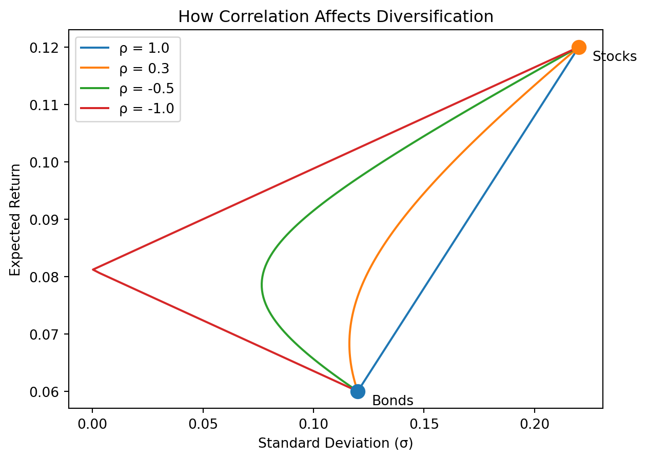

With \(\rho = 1\) (perfect correlation), there’s no diversification benefit — the opportunity set is a straight line between the two assets. As correlation decreases, the curve bends to the left, meaning you can achieve the same expected return with less risk. At \(\rho = -1\) (perfect negative correlation), you can theoretically eliminate all risk by choosing the right combination. In practice, correlations between stocks are positive (typically 0.2–0.5), so diversification helps but doesn’t eliminate risk entirely.

6.4 The Efficient Frontier

With multiple risky assets, different portfolio combinations offer different risk-return profiles. The efficient frontier is the set of portfolios offering the highest expected return for each level of risk. Equivalently, it’s the portfolios offering the lowest risk for each level of expected return.

# Two assets: bonds and stocks
mu_bonds, sigma_bonds = 0.06, 0.12
mu_stocks, sigma_stocks = 0.12, 0.22
rho = 0.3  # correlation

# Generate frontier by varying weights
weights = np.linspace(-0.5, 1.5, 100)
mus = []
sigmas = []

for w in weights:
    mu_p = w * mu_stocks + (1 - w) * mu_bonds
    var_p = (w * sigma_stocks)**2 + ((1-w) * sigma_bonds)**2 + 2*w*(1-w)*rho*sigma_bonds*sigma_stocks
    mus.append(mu_p)
    sigmas.append(np.sqrt(var_p))

# Find minimum variance point
min_var_idx = np.argmin(sigmas)

fig, ax = plt.subplots()
ax.plot(sigmas[:min_var_idx], mus[:min_var_idx], 'r--', label='Inefficient')
ax.plot(sigmas[min_var_idx:], mus[min_var_idx:], 'b-', linewidth=2, label='Efficient Frontier')
ax.scatter([sigma_bonds], [mu_bonds], s=100, zorder=5, label='Bonds')
ax.scatter([sigma_stocks], [mu_stocks], s=100, zorder=5, label='Stocks')
ax.set_xlabel('Standard Deviation')
ax.set_ylabel('Expected Return')
ax.set_title('The Efficient Frontier')
ax.legend()
plt.show()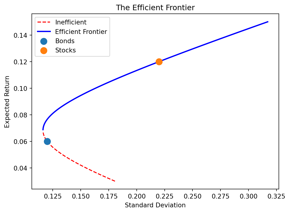

The curve bulges to the left—this is diversification at work. By combining stocks and bonds (which aren’t perfectly correlated), you can achieve lower risk than either asset alone at intermediate return levels. The upper portion (solid blue) is efficient; the lower portion (dashed red) is inefficient—you could get the same return with less risk by moving to the upper branch.

Rational investors should only hold portfolios on the efficient frontier. Given any portfolio below the frontier, you can find one on the frontier that’s strictly better (higher return for the same risk, or lower risk for the same return).

6.5 Estimation with Multiple Assets

Everything above assumes we know the true parameters \(\boldsymbol{\mu}\) and \(\boldsymbol{\Sigma}\). In practice, we estimate them from \(T\) observations of the return vector \(\mathbf{r}_t\):

\[\hat{\boldsymbol{\mu}} = \frac{1}{T} \sum_{t=1}^{T} \mathbf{r}_t \qquad \hat{\boldsymbol{\Sigma}} = \frac{1}{T-1} \sum_{t=1}^{T} (\mathbf{r}_t - \hat{\boldsymbol{\mu}})(\mathbf{r}_t - \hat{\boldsymbol{\mu}})^\prime\]

The sample mean vector \(\hat{\boldsymbol{\mu}}\) has \(N\) elements and the sample covariance matrix \(\hat{\boldsymbol{\Sigma}}\) has \(N(N+1)/2\) unique elements (since it’s symmetric). With 25 assets, that’s 25 means and 325 covariance parameters — all estimated from the same \(T\) observations. The plug-in portfolio substitutes these estimates into the MVO formula:

\[\hat{\mathbf{w}} = \frac{1}{\gamma} \hat{\boldsymbol{\Sigma}}^{-1} \hat{\boldsymbol{\mu}}\]

This is the portfolio you’d actually compute in practice. The question — which we quantified earlier as a utility loss of \(N/(2\gamma T)\) — is how much you lose compared to the true optimum \(\mathbf{w}^*\).

7 Sample vs Population Frontier

7.1 Two Different Frontiers

Plugging in \(\hat{\boldsymbol{\mu}}\) and \(\hat{\boldsymbol{\Sigma}}\) in place of the true parameters produces a different efficient frontier than the one we’d compute with perfect knowledge. This creates two distinct frontiers:

Population frontier: The efficient frontier computed using the true parameters \(\boldsymbol{\mu}\) and \(\boldsymbol{\Sigma}\). This is what we’d see if we had perfect knowledge—the actual investment opportunities available.

Sample frontier: The efficient frontier computed using estimated parameters \(\hat{\boldsymbol{\mu}}\) and \(\hat{\boldsymbol{\Sigma}}\). This is what we actually compute from historical data—our best guess at the opportunities.

Kan and Smith (2008, Management Science) studied the relationship between these frontiers in depth. Their finding is sobering: the sample frontier systematically overstates the true investment opportunities.

7.2 Why Is the Sample Frontier Too Optimistic?

The sample frontier uses estimated parameters that are “tuned” to the historical data. By pure chance, some assets had unusually high returns in the sample period, or unusually low correlations with other assets. The sample frontier exploits these patterns, constructing portfolios that look great on paper.

But these patterns are partly noise. The assets that happened to do well in the sample won’t necessarily do well going forward. The correlations that happened to be low might be higher in the future. When we invest using sample-optimal weights, we’re likely to be disappointed because the estimated patterns don’t persist perfectly.

This is in-sample optimization—exactly the same phenomenon we saw in regression. In Week 5, we learned that a regression model’s in-sample R² overstates its out-of-sample predictive power because the model fits both the signal and the noise in the training data. Portfolio optimization has the same problem: the sample-optimal portfolio is optimized for the sample, not for the future.

The optimizer doesn’t know that some of the patterns in \(\hat{\boldsymbol{\mu}}\) are noise—it treats them as real opportunities and exploits them aggressively. Assets that were lucky get overweighted; assets that were unlucky get underweighted or shorted. This is overfitting applied to portfolio construction.

# Simulate the gap between sample and population frontiers
np.random.seed(42)
N = 10
T = 60  # 5 years of monthly data

# True parameters
true_mu = np.array([0.02 + 0.01 * i for i in range(N)])
true_sigma = np.array([0.10 + 0.015 * i for i in range(N)])
corr = 0.3 * np.ones((N, N)) + 0.7 * np.eye(N)
true_Sigma = np.outer(true_sigma, true_sigma) * corr

# Generate sample
returns = np.random.multivariate_normal(true_mu, true_Sigma, T)
sample_mu = returns.mean(axis=0)
sample_Sigma = np.cov(returns, rowvar=False)

# Function to compute frontier points
def frontier_points(mu, Sigma, weights_range):
    gmv_w = np.linalg.solve(Sigma, np.ones(len(mu)))
    gmv_w = gmv_w / gmv_w.sum()
    tangency_w = np.linalg.solve(Sigma, mu)
    tangency_w = tangency_w / tangency_w.sum()

    sigmas, mus = [], []
    for a in weights_range:
        w = a * tangency_w + (1 - a) * gmv_w
        sigmas.append(np.sqrt(w @ Sigma @ w))
        mus.append(w @ mu)
    return sigmas, mus

weights_range = np.linspace(0, 2, 50)
true_sigmas, true_mus = frontier_points(true_mu, true_Sigma, weights_range)
sample_sigmas, sample_mus = frontier_points(sample_mu, sample_Sigma, weights_range)

fig, ax = plt.subplots()
ax.plot(true_sigmas, true_mus, 'b-', linewidth=2, label='True Frontier')
ax.plot(sample_sigmas, sample_mus, 'r--', linewidth=2, label='Sample Frontier')
ax.set_xlabel('Standard Deviation')
ax.set_ylabel('Expected Return')
ax.set_title('Sample Frontier Overstates Opportunities (T=60, N=10)')
ax.legend()
plt.show()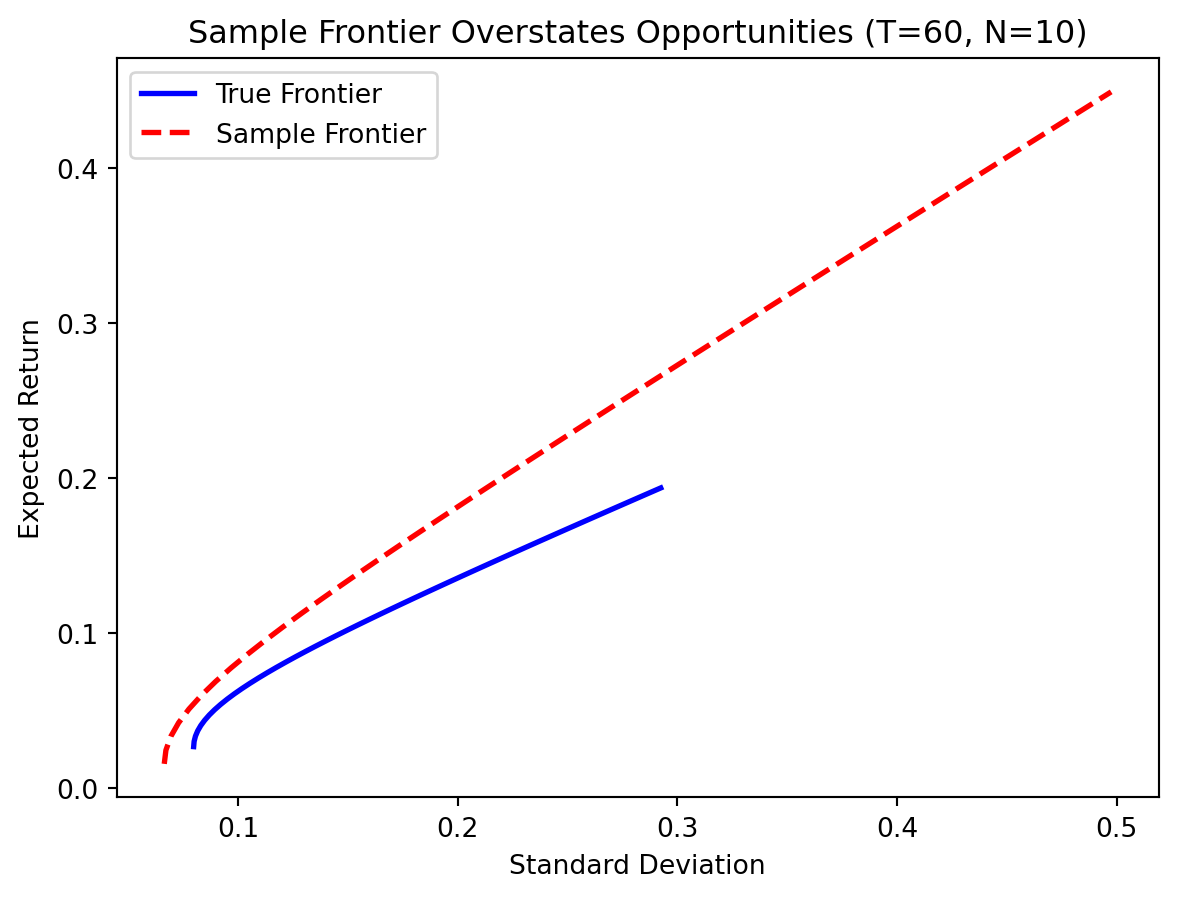

The sample frontier (red dashed) lies above and to the left of the true frontier (blue solid)—it promises higher returns for less risk. But this is an illusion. When you actually invest using the sample-optimal weights, you’ll earn returns consistent with the true frontier, not the sample frontier.

7.3 Out-of-Sample Performance

What happens when we actually invest based on sample-optimal weights? We can simulate this: estimate the tangency portfolio from one sample, then evaluate it on a fresh sample drawn from the same distribution. The in-sample Sharpe ratio (computed from the estimation data) tells us what the optimizer promises; the out-of-sample Sharpe ratio (computed from new data) tells us what we actually get.

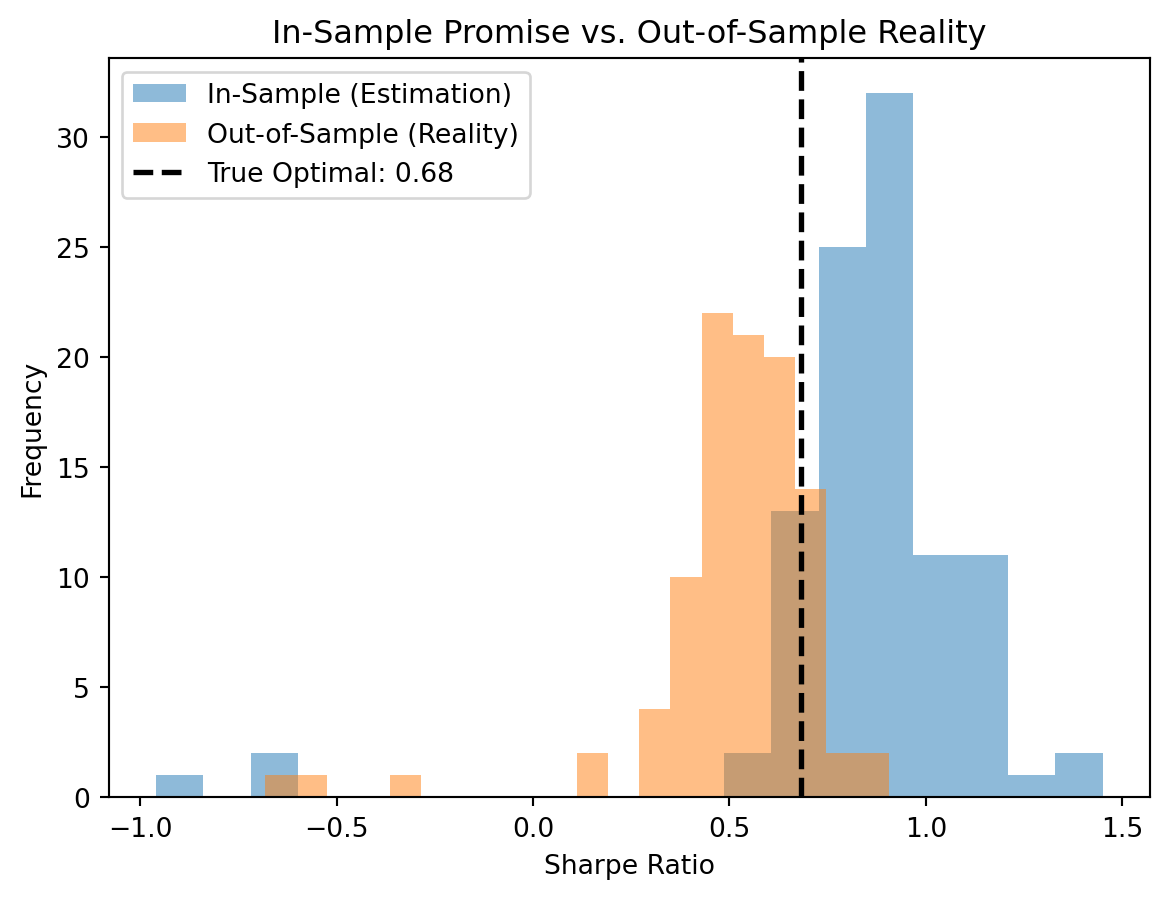
The in-sample Sharpe ratios cluster well above the true optimal Sharpe ratio — the optimizer is overfitting to sample noise, making the portfolio look better than it is. The out-of-sample Sharpe ratios are much lower, often falling below the true optimum. This is the portfolio analog of training-set R² overstating test-set performance.

7.4 The Effect of Sample Size

The gap between sample and population frontiers depends on how much data you have:

• Large \(T\) relative to \(N\): The sample frontier is close to the true frontier. Estimates are precise, and optimization doesn’t overfit much.
• Small \(T\) relative to \(N\): The sample frontier is wildly optimistic. Estimates are noisy, and the optimizer exploits noise as if it were signal.
• \(T\) close to \(N\): The sample covariance matrix becomes nearly singular (hard to invert), and portfolio weights become extreme and unstable.

When \(N\) approaches \(T\), the problem becomes pathological. The sample covariance matrix has \(N(N+1)/2\) unique elements to estimate from only \(NT\) data points. When \(N = T\), you have exactly as many parameters as observations—classic overfitting territory.

This is exactly like regression with too many predictors relative to observations. In regression, we learned that when \(p > n\), OLS doesn’t even have a unique solution. The portfolio analog is that when \(N > T\), the sample covariance matrix is singular and can’t be inverted at all.

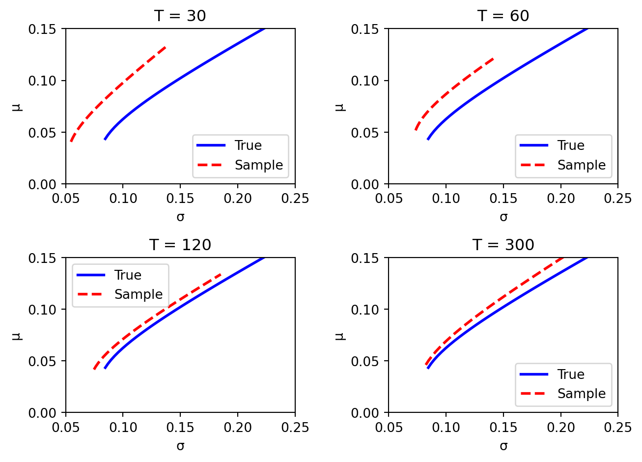
With little data (\(T = 30\)), the sample frontier is far from the truth. As \(T\) increases, the sample frontier converges toward the population frontier, but the convergence is slow — even at \(T = 300\) (25 years of monthly data), a visible gap remains.

8 Dealing with Estimation Risk

8.1 Approaches to Reduce Estimation Risk

Given the severity of estimation risk, researchers have proposed many strategies to improve portfolio performance:

1. Avoid optimization altogether: Use simple rules like equal weights (\(w_i = 1/N\))
2. Impose structure: Use factor models to reduce the number of parameters
3. Add constraints: Short-selling restrictions or bounds on individual weights
4. Target minimum variance: The GMV portfolio doesn’t depend on estimated expected returns
5. Combine portfolios optimally: Blend the tangency and minimum variance portfolios
6. Use regularization: Apply ML techniques like Lasso to shrink unstable weights

Each approach trades off different concerns. Let’s examine the most important ones.

8.2 The 1/N Portfolio

The simplest approach: invest equally in all assets. \[w_i = \frac{1}{N} \quad \text{for all } i\]

No estimation required! You don’t need to know expected returns or covariances—just divide your money equally. This seems naive, even foolish. Surely sophisticated optimization should beat such a simple rule?

DeMiguel, Garlappi, and Uppal (2009) compared 14 sophisticated portfolio optimization strategies to 1/N using real data across multiple asset classes and time periods. Their finding:

None of the optimized portfolios consistently outperformed 1/N out of sample.

This is a remarkable result. Decades of portfolio theory—mean-variance optimization, Bayesian approaches, shrinkage estimators, robust optimization—and none of it reliably beats dividing your money equally. The reason? Estimation error overwhelms the benefits of optimization.

The theoretical optimal portfolio is indeed better than 1/N—if you knew the true parameters. But you don’t. The gap between the sample-optimal portfolio and the true optimal portfolio is often larger than the gap between 1/N and the true optimal portfolio. Simple rules are more robust because they don’t try to exploit patterns that might be noise.

8.3 The Global Minimum Variance Portfolio

Another robust option: the global minimum variance (GMV) portfolio — the portfolio with the lowest possible variance among all portfolios that are fully invested in risky assets. \[\mathbf{w}_{\text{GMV}} = \frac{\boldsymbol{\Sigma}^{-1} \mathbf{1}}{\mathbf{1}^\prime \boldsymbol{\Sigma}^{-1} \mathbf{1}}\]

where \(\mathbf{1}\) is a vector of ones (ensuring the weights sum to 1). Geometrically, the GMV portfolio is the vertex of the efficient frontier — the leftmost point, where risk is minimized regardless of return.

The GMV portfolio has a special property: it doesn’t depend on estimated expected returns — only on the covariance matrix \(\boldsymbol{\Sigma}\). This is a major advantage because:

• Expected returns are extremely hard to estimate (the signal-to-noise problem)
• Covariances are estimated much more precisely than means
• Removing \(\hat{\boldsymbol{\mu}}\) from the optimization removes a major source of estimation error

Empirically, the GMV portfolio often outperforms the tangency portfolio out of sample, despite being theoretically suboptimal. It sacrifices some expected return but gains substantially in stability.

# GMV portfolio: vertex of the efficient frontier
# w_1_20 = Σ⁻¹1 / 1'Σ⁻¹1 (computed in the frontier code above)
gmv_ret = w_1_20 @ mu_20
gmv_vol = np.sqrt(w_1_20 @ Sigma_20 @ w_1_20)

fig, ax = plt.subplots()

# Individual stocks
ax.scatter(vols_20, mu_20, s=30, zorder=3)
for i, t in enumerate(tickers):
    ax.annotate(t, (vols_20[i], mu_20[i]), fontsize=6, ha='center', va='bottom')

# Efficient frontier
ax.plot(eff_vols_20, target_rets_20, linewidth=2, label='Efficient frontier')

# GMV portfolio
ax.scatter([gmv_vol], [gmv_ret], s=150, marker='D', zorder=5,
           label='Global Minimum Variance (GMV)')

ax.set_xlabel('Risk (standard deviation)')
ax.set_ylabel('Expected return')
ax.set_title('The GMV Portfolio: Vertex of the Efficient Frontier')
ax.legend(loc='lower right')
plt.show()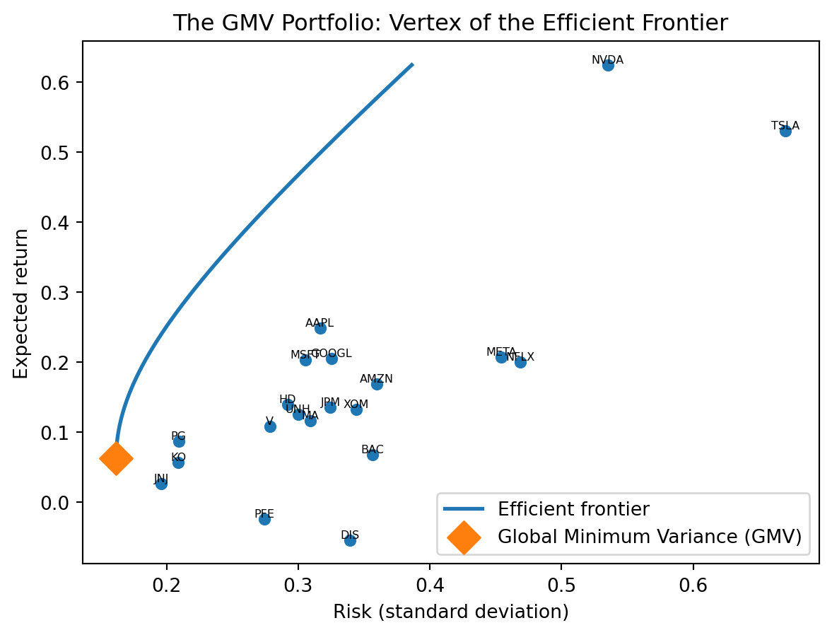

8.4 Regularization: The ML Connection

Here’s where machine learning enters portfolio optimization directly. The overfitting problem in portfolios is fundamentally the same as in regression—we’re fitting too aggressively to noisy data. And the solution is the same: regularization.

Recall from Week 5 that Lasso regression adds a penalty for large coefficients: \[\text{Lasso:} \quad \min_{\boldsymbol{\beta}} \sum_{i=1}^{n} (y_i - \hat{y}_i)^2 + \lambda \sum_{j=1}^{p} |\beta_j|\]

The penalty \(\lambda \sum_j |\beta_j|\) shrinks coefficients toward zero, preventing the model from exploiting noise in the training data.

The same idea applies to portfolio weights: \[\text{Regularized Portfolio:} \quad \min_{\mathbf{w}} \left(\text{portfolio variance}\right) + \lambda \|\mathbf{w}\|_1\]

where \(\|\mathbf{w}\|_1 = \sum_i |w_i|\) is the sum of absolute weights.

This penalizes extreme positions. Small weights shrink to exactly zero (sparse portfolios), and large weights are pulled back toward moderate values. The result is a portfolio that doesn’t try to exploit every estimated pattern, only the strongest ones.

8.5 From MVO to Regression

The central problem of this chapter is that the MVO solution \(\mathbf{w}^* = \frac{1}{\gamma}\boldsymbol{\Sigma}^{-1}\boldsymbol{\mu}\) requires inverting \(\hat{\boldsymbol{\Sigma}}\), which is unstable when \(N\) is large relative to \(T\). Ao, Li, and Zheng (2019, Review of Financial Studies) found a way to sidestep this entirely by recasting the problem as a regression.

Start with the standard mean-variance problem: maximize expected return for a given risk budget \(\sigma\):

\[\arg\max_{\mathbf{w}} \; \mathbf{w}^\prime \boldsymbol{\mu} \quad \text{subject to} \quad \mathbf{w}^\prime \boldsymbol{\Sigma} \mathbf{w} \leq \sigma^2\]

The explicit solution is \(\mathbf{w}^* = \frac{\sigma}{\sqrt{\theta}}\boldsymbol{\Sigma}^{-1}\boldsymbol{\mu}\), where \(\theta = \boldsymbol{\mu}^\prime\boldsymbol{\Sigma}^{-1}\boldsymbol{\mu}\) is the squared Sharpe ratio of the optimal (tangency) portfolio — the same quantity we wrote as \(\theta^2\) in the single-asset case. (Ao et al. use a single \(\theta\) for the squared Sharpe ratio, so we follow their convention for the rest of this section.) This solution requires the matrix inverse \(\boldsymbol{\Sigma}^{-1}\) — exactly the operation that blows up with noisy estimates.

Ao, Li, and Zheng prove that this same \(\mathbf{w}^*\) also solves an unconstrained regression problem:

\[\mathbf{w}^* = \arg\min_{\mathbf{w}} \; \mathbb{E}\left[(r_c - \mathbf{w}^\prime \mathbf{r}_t)^2\right], \qquad r_c = \sigma \cdot \frac{1 + \theta}{\sqrt{\theta}}\]

The constant \(r_c\) bundles your risk budget \(\sigma\) and the market’s Sharpe ratio \(\theta\) into a single target. Different values of \(r_c\) correspond to different points on the efficient frontier — just like choosing different \(\gamma\) in MVO or different \(\sigma\) in the constrained problem. The regression asks: find the portfolio whose return tracks a constant \(r_c\) as closely as possible. Same answer as the constrained optimization — but now it’s a regression, with no matrix inversion and no constraints.

8.6 MAXSER: Estimating \(r_c\) and Running Lasso

The regression formulation requires \(r_c = \sigma \frac{1+\theta}{\sqrt{\theta}}\), which depends on \(\theta = \boldsymbol{\mu}^\prime\boldsymbol{\Sigma}^{-1}\boldsymbol{\mu}\) — the thing we’re trying to estimate in the first place. So we need an estimate \(\hat{\theta}\).

The plug-in (sample) estimate is \(\hat{\theta}_s = \hat{\boldsymbol{\mu}}^\prime \hat{\boldsymbol{\Sigma}}^{-1} \hat{\boldsymbol{\mu}}\), but this is heavily biased upward when \(N/T\) isn’t negligible — the same estimation-risk problem from earlier. So we use the bias-corrected estimator from Kan and Zhou (2007):

\[\hat{\theta} = \frac{(T - N - 2)\,\hat{\theta}_s - N}{T}\]

Ao et al. use a further adjusted version to ensure \(\hat{\theta}\) stays non-negative. Once you have \(\hat{\theta}\), you compute \(\hat{r}_c\) and run Lasso:

\[\hat{\mathbf{w}}_{\text{MAXSER}} = \arg\min_{\mathbf{w}} \frac{1}{T} \sum_{t=1}^{T} (\hat{r}_c - \mathbf{w}^\prime \mathbf{r}_t)^2 + \lambda \|\mathbf{w}\|_1\]

This is MAXSER — Maximum Sharpe Ratio Estimated by Sparse Regression. Cross-validation picks \(\lambda\), just like in standard Lasso.

A natural question: doesn’t computing \(\hat{\theta}_s = \hat{\boldsymbol{\mu}}'\hat{\boldsymbol{\Sigma}}^{-1}\hat{\boldsymbol{\mu}}\) still require inverting \(\hat{\boldsymbol{\Sigma}}\)? It does — but there’s a crucial difference. In plug-in MVO, \(\hat{\boldsymbol{\Sigma}}^{-1}\hat{\boldsymbol{\mu}}\) produces an \(N\)-dimensional weight vector: errors in the inverse get amplified along poorly-estimated eigenvectors, fanning out into extreme positions across all \(N\) assets. In MAXSER, \(\hat{\boldsymbol{\mu}}'\hat{\boldsymbol{\Sigma}}^{-1}\hat{\boldsymbol{\mu}}\) produces a single scalar \(\hat{\theta}_s\). The same noisy inverse is involved, but the errors collapse into one number rather than \(N\) unstable weights. That scalar is biased upward — but the bias is well-characterized and correctable (the Kan–Zhou formula above).

Once you have \(\hat{r}_c\), the actual weight estimation is pure Lasso on the raw return vectors \(\mathbf{r}_t\) — no matrix inversion needed. The covariance matrix doesn’t need to be explicitly estimated or inverted for the weight step. The regularization penalty \(\lambda\|\mathbf{w}\|_1\) does the work that a stable matrix inversion would do: it controls the complexity of the solution and prevents the weights from exploiting noise. In short, the matrix inverse is quarantined to estimating a single correctable scalar, rather than directly determining all \(N\) portfolio weights.

8.7 What MAXSER Gives You

MAXSER estimates a single portfolio: the tangency portfolio — the risky-asset portfolio with the highest Sharpe ratio. Recall from the efficient frontier discussion that once you have the tangency, every investor just mixes it with the risk-free asset along the CAL. Risk aversion \(\gamma\) determines how far along the line you go. So estimating the tangency well is the whole game.

The plug-in tangency (\(\hat{\boldsymbol{\Sigma}}^{-1}\hat{\boldsymbol{\mu}}\), normalized) uses all \(N\) assets with wildly unstable weights. It achieves a high in-sample Sharpe ratio, but this is overfitting: the optimizer exploits sample noise. Out of sample, the portfolio disappoints.

The MAXSER tangency (Lasso regression with bias-corrected \(\hat{r}_c\), normalized) sets most weights to exactly zero, investing in a sparse subset. The remaining weights are shrunk, preventing extreme positions. It achieves a lower in-sample Sharpe ratio (honestly so), but is more stable and often performs better out of sample.

This is overfitting vs. regularization — the same trade-off from Week 5, now applied to portfolios.

8.8 Choosing the Regularization Parameter

How do we choose the penalty \(\lambda\) in MAXSER? Three approaches:

1. Cross-validation to maximize out-of-sample Sharpe ratio. Split the data into folds, fit the Lasso for each candidate \(\lambda\) on the training folds, evaluate portfolio Sharpe ratio on the held-out fold, and choose the \(\lambda\) that gives the best out-of-sample performance. This is the most direct approach.

2. Cross-validation to match a target risk level. Instead of maximizing the Sharpe ratio, choose \(\lambda\) so the portfolio’s out-of-sample volatility matches a desired risk budget \(\sigma\).

3. Bias-corrected Sharpe ratio estimator. Use an analytical correction (like the Kan and Zhou adjustment) rather than cross-validation. This avoids the computational cost of repeated fitting but requires distributional assumptions.

In practice, the cross-validation approach is most common — it’s exactly the procedure from Week 5 applied to a portfolio objective instead of mean squared error.

8.9 Summary of Approaches

Method	Advantages	Disadvantages
1/N	No estimation, simple, robust	Ignores all information in the data
GMV	Ignores noisy means, more stable	Suboptimal if means are actually predictable
Constraints	Intuitive bounds on positions	Ad hoc, may over-constrain unnecessarily
MAXSER (Lasso)	Principled, sparse, stable	Requires tuning \(\lambda\) via cross-validation

The ML approach provides a principled way to balance competing goals: using information in the data (through estimation) without overfitting (through regularization). It’s not magic—regularized portfolios still underperform the theoretical optimum you’d achieve with perfect knowledge. But they come closer than plug-in estimators that ignore estimation error.

9 Summary

Mean-variance utility provides a framework for ranking portfolios: \(U = \mu_p - \frac{\gamma}{2}\sigma_p^2\). Investors like expected return and dislike variance, with the risk aversion parameter \(\gamma\) determining the trade-off.

Optimal portfolios maximize utility. With one risky asset: \(w^* = \frac{\mu}{\gamma\sigma^2}\). With multiple assets: \(\mathbf{w}^* = \frac{1}{\gamma}\boldsymbol{\Sigma}^{-1}\boldsymbol{\mu}\). These formulas are elegant but require knowing true parameters.

The estimation problem: We don’t know true parameters—we estimate them from data. Even with 98 years of stock market history, the 95% confidence interval for expected return spans roughly 4.5% to 12.5%. This enormous uncertainty flows directly into uncertainty about optimal weights.

Utility loss from estimation: Using estimated weights instead of true optimal weights costs utility. With \(N\) assets: \[\text{Utility Loss} = \frac{N}{2\gamma T}\]

The loss grows with more assets—the curse of dimensionality. With 25 assets and 5 years of data, estimation error can wipe out most of the theoretical benefits of optimization.

Sample vs population frontier: The efficient frontier computed from historical data systematically overstates the true investment opportunities. The sample-optimal portfolio looks great on paper but disappoints in practice—this is overfitting applied to portfolio construction.

Dealing with estimation risk: Simple approaches like 1/N and the GMV portfolio often beat sophisticated optimization because they don’t try to exploit noisy estimates. ML techniques like Lasso (MAXSER) provide a principled middle ground — using information while controlling overfitting.

The ML connection: Ao, Li, and Zheng (2019) showed that the mean-variance portfolio problem can be recast as a regression: the optimal portfolio weights are regression coefficients predicting a target constant \(r_c\) from asset returns. This converts the unstable matrix-inversion problem into a standard regression, where we can directly apply Lasso regularization and cross-validation — the same tools from Week 5. MAXSER demonstrates that ML isn’t just for prediction but also for decision-making under uncertainty.

Next week: We move from regression (continuous outcomes) to classification (categorical outcomes): predicting which category an observation belongs to. Will a firm default? Which way will the market move? Classification is another core supervised learning problem with many applications in finance.

10 References

• Ao, M., Li, Y., & Zheng, X. (2019). Approaching mean-variance efficiency for large portfolios. Review of Financial Studies, 32(7), 2890–2919.
• DeMiguel, V., Garlappi, L., & Uppal, R. (2009). Optimal versus naive diversification: How inefficient is the 1/N portfolio strategy? Review of Financial Studies, 22(5), 1915–1953.
• Goyal, A., & Welch, I. (2008). A comprehensive look at the empirical performance of equity premium prediction. Review of Financial Studies, 21(4), 1455–1508.
• Kan, R., & Smith, D. R. (2008). The distribution of the sample minimum-variance frontier. Management Science, 54(7), 1364–1380.
• Kan, R., & Zhou, G. (2007). Optimal portfolio choice with parameter uncertainty. Journal of Financial and Quantitative Analysis, 42(3), 621–656.
• Markowitz, H. (1952). Portfolio selection. Journal of Finance, 7(1), 77–91.

Week 5: Regression

More chapters coming soon