If \(|z_1| > 1.96\) or \(|z_2| > 1.96\), reject normality at 5% level.
Empirical Evidence: S&P 500 Returns
import numpy as npimport pandas as pdfrom scipy import statsimport os# Load S&P 500 data (cache locally to avoid repeated downloads)csv_path ='sp500_yf.csv'if os.path.exists(csv_path): sp500 = pd.read_csv(csv_path, index_col='Date', parse_dates=True)else:import yfinance as yf sp500 = yf.download('^GSPC', start='1950-01-01', end='2025-12-31', progress=False) sp500.columns = sp500.columns.get_level_values(0) # Flatten multi-level columns sp500.to_csv(csv_path)# Compute daily log returnssp500['log_return'] = np.log(sp500['Close'] / sp500['Close'].shift(1))returns = sp500['log_return'].dropna()# Date rangeprint(f"Data range: {returns.index.min().strftime('%Y-%m-%d')} to {returns.index.max().strftime('%Y-%m-%d')}")print(f"Number of daily observations: T = {len(returns):,}")# Summary statisticsmean_ret = returns.mean()std_ret = returns.std()skew = stats.skew(returns)kurt = stats.kurtosis(returns) # excess kurtosisprint(f"\nSample mean (daily): {mean_ret:.4%}")print(f"Sample std dev (daily): {std_ret:.4%}")print(f"Skewness: {skew:.3f}")print(f"Excess kurtosis: {kurt:.2f}")# Test statisticsT =len(returns)z1 = skew / np.sqrt(6/T)z2 = kurt / np.sqrt(24/T)print(f"\nTest statistics:")print(f"z_skewness = {z1:.2f} (reject if |z| > 1.96)")print(f"z_kurtosis = {z2:.2f} (reject if |z| > 1.96)")
Data range: 1950-01-04 to 2025-12-17
Number of daily observations: T = 19,111

Sample mean (daily): 0.0314%
Sample std dev (daily): 0.9970%
Skewness: -0.952
Excess kurtosis: 25.28

Test statistics:
z_skewness = -53.76  (reject if |z| > 1.96)
z_kurtosis = 713.24  (reject if |z| > 1.96)
Conclusion: Skewness is significantly negative (left tail), and kurtosis is way too high. Stock returns have fat tails—they are not normally distributed.
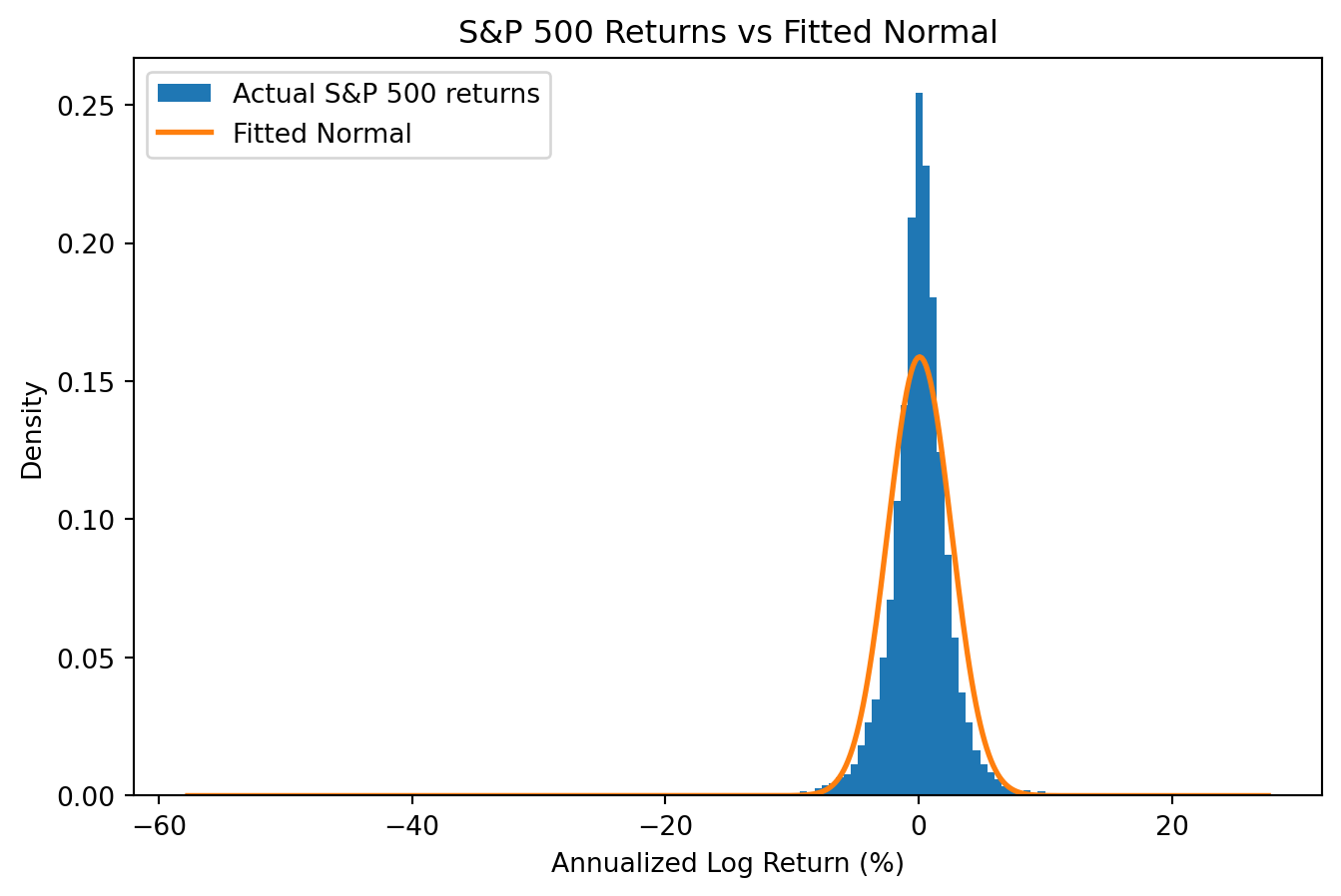
S&P 500 Returns vs the Fitted Normal Distribution
import numpy as npimport pandas as pdimport matplotlib.pyplot as pltfrom scipy import statsimport os# Load S&P 500 data (cache locally to avoid repeated downloads)csv_path ='sp500_yf.csv'if os.path.exists(csv_path): sp500 = pd.read_csv(csv_path, index_col='Date', parse_dates=True)else:import yfinance as yf sp500 = yf.download('^GSPC', start='1950-01-01', end='2025-12-31', progress=False) sp500.columns = sp500.columns.get_level_values(0) # Flatten multi-level columns sp500.to_csv(csv_path)sp500['log_return'] = np.log(sp500['Close'] / sp500['Close'].shift(1))returns = sp500['log_return'].dropna()# Annualize: multiply by 252 trading daysreturns_annual = returns *252# Fit a normal distribution using sample mean and std devmu_hat = returns_annual.mean()sigma_hat = returns_annual.std()# Plot histogram of actual returns (log scale on y-axis)fig, ax = plt.subplots(figsize=(8, 5))ax.hist(returns_annual, bins=150, density=True, label='Actual S&P 500 returns')# Overlay the FITTED normal distribution (same mean and std dev)x = np.linspace(returns_annual.min(), returns_annual.max(), 500)ax.plot(x, stats.norm.pdf(x, mu_hat, sigma_hat), label='Fitted Normal', linewidth=2)ax.set_xlabel('Annualized Log Return (%)')ax.set_ylabel('Density')ax.legend()ax.set_title('S&P 500 Returns vs Fitted Normal')plt.show()# Count extreme events (using daily standardized returns)standardized = (returns - returns.mean()) / returns.std()n_extreme = (abs(standardized) >4).sum()expected_normal =len(returns) *2* stats.norm.sf(4) # two-tailedprint(f"Observations beyond 4 std devs: {n_extreme}")print(f"Normal distribution predicts: {expected_normal:.1f}")print(f"Actual is {n_extreme/expected_normal:.0f}x more than expected!")
Observations beyond 4 std devs: 107
Normal distribution predicts: 1.2
Actual is 88x more than expected!
Box Plots: Actual vs Normal-Implied Returns
import numpy as npimport pandas as pdimport matplotlib.pyplot as pltimport os# Load S&P 500 data (cache locally to avoid repeated downloads)csv_path ='sp500_yf.csv'if os.path.exists(csv_path): sp500 = pd.read_csv(csv_path, index_col='Date', parse_dates=True)else:import yfinance as yf sp500 = yf.download('^GSPC', start='1950-01-01', end='2025-12-31', progress=False) sp500.columns = sp500.columns.get_level_values(0) # Flatten multi-level columns sp500.to_csv(csv_path)sp500['log_return'] = np.log(sp500['Close'] / sp500['Close'].shift(1))returns = sp500['log_return'].dropna()# Annualizereturns_annual = returns *252# Simulate from a normal with the same mean and std devnp.random.seed(42)normal_sim = np.random.normal(returns_annual.mean(), returns_annual.std(), len(returns_annual))# Side-by-side box plotsfig, ax = plt.subplots(figsize=(6, 5))ax.boxplot([returns_annual, normal_sim], labels=['Actual S&P 500', 'Normal (simulated)'])ax.set_ylabel('Annualized Daily Log Return (%)')ax.set_title('Box Plot Comparison: Fat Tails in Action')ax.axhline(0, linestyle='--', linewidth=0.5)plt.show()
The actual returns have far more outliers (the dots beyond the whiskers) than a normal distribution with the same mean and variance would produce.
Quantifying the Fat Tails
import numpy as npimport pandas as pdfrom scipy import statsimport os# Load S&P 500 datacsv_path ='sp500_yf.csv'sp500 = pd.read_csv(csv_path, index_col='Date', parse_dates=True)sp500['log_return'] = np.log(sp500['Close'] / sp500['Close'].shift(1))returns = sp500['log_return'].dropna()# Standardize returnsmu, sigma = returns.mean(), returns.std()standardized = (returns - mu) / sigma# Count extreme events at various thresholdsfor k in [3, 4, 5, 6]: actual = (abs(standardized) > k).sum() expected =len(returns) *2* stats.norm.sf(k) # two-tailed ratio = actual / expected if expected >0else np.infprint(f"{k}-sigma events: {actual} actual vs {expected:.2e} expected → {ratio:,.0f}× more")# Find the worst day (Black Monday: October 19, 1987)worst_day = returns.idxmin()worst_return = returns.min()worst_sigma = (worst_return - mu) / sigmaprint(f"\nWorst day: {worst_day.strftime('%Y-%m-%d')}")print(f"Return: {worst_return:.2%}")print(f"Standard deviations from mean: {worst_sigma:.1f} sigma")# Probability of this under normalityprob_normal =2* stats.norm.sf(abs(worst_sigma))print(f"Probability under normality: {prob_normal:.2e}")print(f"That's 1 in {1/prob_normal:.2e} days")
3-sigma events: 272 actual vs 5.16e+01 expected → 5× more
4-sigma events: 107 actual vs 1.21e+00 expected → 88× more
5-sigma events: 53 actual vs 1.10e-02 expected → 4,837× more
6-sigma events: 35 actual vs 3.77e-05 expected → 928,152× more

Worst day: 1987-10-19
Return: -22.90%
Standard deviations from mean: -23.0 sigma
Probability under normality: 4.53e-117
That's 1 in 2.21e+116 days
Summary: The Normality Assumption
Key findings from 75 years of S&P 500 daily returns:
Mean and volatility are reasonable: ~8% annual return, ~16% annual volatility
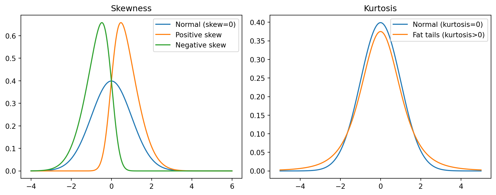
Negative skewness (\(\approx -1\)): Crashes are sharper than rallies
Excess kurtosis \(\approx 25\): Extreme events are far more common than normal predicts
Why do the test statistics look so extreme?
With \(T \approx 19{,}000\) daily observations, the standard error is tiny (\(\approx 1/\sqrt{T}\)). Even modest departures from normality become statistically overwhelming. This is the point: we have decisive evidence against normality.
Practical implication:
The normal distribution works fine for “typical” days. But it dangerously underestimates tail risk—4-sigma events happen 88× more often than normality predicts. Black Monday (1987) was a 23-sigma event: probability \(\approx 10^{-117}\) under normality. Yet it happened.
Part II: Autocorrelation
Does Yesterday Predict Today?
So far we’ve implicitly assumed returns are independent over time—yesterday’s return tells us nothing about today’s.
Autocorrelation (also called serial correlation) measures the extent to which a variable is correlated with its own past values.
Positive autocorrelation: High returns tend to be followed by high returns (momentum)
Negative autocorrelation: High returns tend to be followed by low returns (reversal)
Zero autocorrelation: Past returns don’t predict future returns
\(\hat{\rho}_1\): Correlation between today’s return and yesterday’s (lag 1)
\(\hat{\rho}_5\): Correlation between today’s return and the return 5 days ago
\(\hat{\rho}_k \in [-1, 1]\) by construction
Under the null hypothesis of no autocorrelation:
\[\hat{\rho}_k \sim N\left(0, \frac{1}{T}\right) \quad \text{approximately, for large } T\]
A 95% confidence interval is roughly \(\pm 2/\sqrt{T}\).
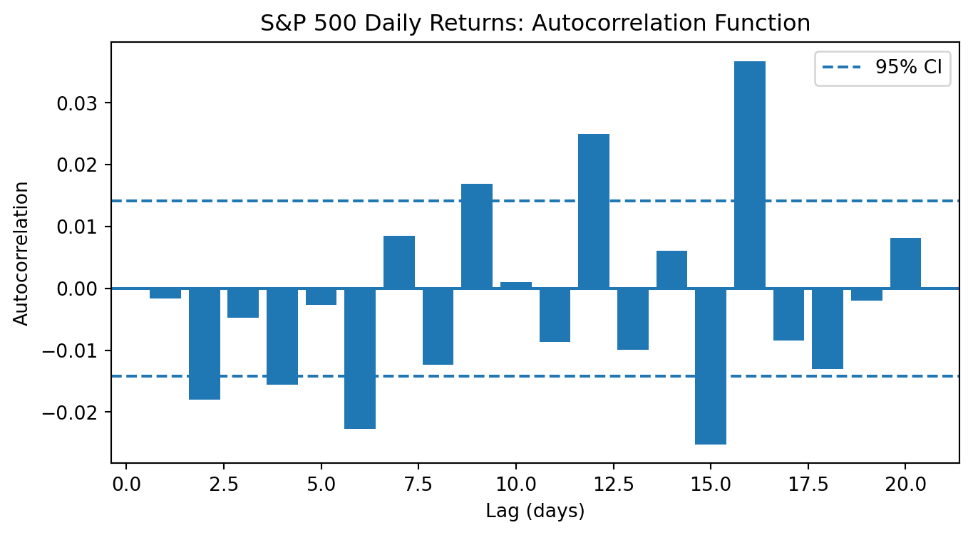
S&P 500 Autocorrelation: Live Data
import numpy as npimport pandas as pdimport os# Load S&P 500 datacsv_path ='sp500_yf.csv'sp500 = pd.read_csv(csv_path, index_col='Date', parse_dates=True)sp500['log_return'] = np.log(sp500['Close'] / sp500['Close'].shift(1))returns = sp500['log_return'].dropna()T =len(returns)print(f"Sample size: T = {T:,}")print(f"Standard error under null: 1/√T = {1/np.sqrt(T):.4f}")print(f"95% CI: ±{1.96/np.sqrt(T):.4f}")# Compute autocorrelations at lags 1-10print(f"\nAutocorrelations:")for k inrange(1, 11): rho_k = returns.autocorr(lag=k) z_stat = rho_k * np.sqrt(T) sig ="*"ifabs(z_stat) >1.96else""print(f" Lag {k:2d}: ρ = {rho_k:+.4f}, z = {z_stat:+.2f}{sig}")
Sample size: T = 19,111
Standard error under null: 1/√T = 0.0072
95% CI: ±0.0142

Autocorrelations:
  Lag  1: ρ = -0.0016, z = -0.22
  Lag  2: ρ = -0.0179, z = -2.48 *
  Lag  3: ρ = -0.0047, z = -0.65
  Lag  4: ρ = -0.0155, z = -2.15 *
  Lag  5: ρ = -0.0027, z = -0.37
  Lag  6: ρ = -0.0227, z = -3.13 *
  Lag  7: ρ = +0.0085, z = +1.18
  Lag  8: ρ = -0.0123, z = -1.70
  Lag  9: ρ = +0.0169, z = +2.33 *
  Lag 10: ρ = +0.0010, z = +0.14
Most lags show tiny autocorrelations—but with \(T \approx 19{,}000\), even tiny correlations can be statistically significant. The economic significance is another matter…
The Ljung-Box Test
Testing autocorrelations one at a time is tedious. The Ljung-Box test tests whether any of the first \(K\) autocorrelations are significantly different from zero.
where \(\mathbf{x}_t = (x_{1,t}, x_{2,t}, \ldots, x_{p,t})'\) is the vector of predictors and \(\boldsymbol{\beta} = (\beta_1, \beta_2, \ldots, \beta_p)'\) is the vector of slopes.
Question: How do we measure whether the predictors actually help?
Answer: The \(R^2\) statistic—but we need to be careful about which\(R^2\).
In-Sample \(R^2\)
The standard in-sample\(R^2\) measures how well the fitted model explains variation in the data used to estimate it:
Interpretation: This is the “guaranteed” return the investor would accept instead of taking on the risk. The term \(\mu^2/(2\gamma\sigma^2)\) is the value of being able to invest in the risky asset.
Certainty Equivalence and Predictability
Key insight: If we can predict returns (\(\mu\) varies over time), we can time the market.
When predicted return is high \(\Rightarrow\) increase \(w\) (invest more)
When predicted return is low \(\Rightarrow\) decrease \(w\) (invest less)
The value of predictability depends on:
How much \(\mu\) varies (more variation = more value)
How well we can forecast (higher \(R^2\) = more value)
Risk aversion \(\gamma\) (affects how aggressively we act on forecasts)
This framework will be central when we evaluate ML prediction models: even a small \(R^2\) improvement can translate into substantial utility gains.
Summary and Looking Ahead
Today’s Key Results
Part I: The Normality Assumption Is Approximate
Returns have fat tails (high kurtosis)
Normal models underestimate extreme events
Part II: Autocorrelation
Weak evidence that past returns predict future returns
Momentum at short horizons, mean reversion at long horizons
Parts III–IV: Predictive Regressions and OOS Testing
In-sample \(R^2\) overstates predictability
Most predictors fail out-of-sample (Goyal-Welch 2008)
Part V: Certainty Equivalence
Even small predictability has economic value
Framework for translating forecasts into portfolio decisions
What’s Next
Week 4: Introduction to Machine Learning
Supervised vs unsupervised learning
The prediction problem: given \(X\), predict \(Y\)
Bias-variance tradeoff
Cross-validation for time series
Preview: ML methods are designed to avoid overfitting and improve out-of-sample performance—exactly what we need for return prediction.
The rest of the course builds on today’s foundations:
Regularization (Weeks 6–7): Fighting overfitting in regression
Classification (Weeks 8–9): Predicting categories, not values