RSM338: Applications of Machine Learning in Finance
Week 2: Financial Data I | January 14–15, 2026
Kevin Mott
Rotman School of Management
Motivation and Overview
Much of quantitative finance—and the ML applications we will study—centers on return prediction.
We model and forecast returns because they have convenient statistical properties.
However, investors ultimately care about wealth: the dollar value of their portfolio.
Wealth is a nonlinear function of returns, which creates a fundamental issue.
In general, for a nonlinear function \(f\) and random variable \(X\): \[\mathbb{E}[f(X)] \neq f(\mathbb{E}[X])\]
As we will see, we usually choose to model log returns: \(r_t = \ln P_{t} - \ln P_{t-1}\)
A standard statistical assumption is that log returns \(r_t\) are normally distributed
What does this imply for the distribution of wealth\(W_t\)? \[ r_t \sim \mathcal N \implies W_t \sim \boxed{\quad\quad\quad} \text{?} \]
This means that knowing the expected return does not directly tell us the expected wealth.
Today we develop the statistical framework for translating between returns and wealth: this is an application of the more general study of random variables.
Part I introduces log returns (continuously compounded returns) and shows that if log returns are normally distributed, then wealth follows a log-normal distribution. We derive the expected value of log-normal wealth and show why it differs systematically from naive forecasts.
Part II addresses estimation risk: when we estimate expected returns from historical data, how does that uncertainty propagate into wealth forecasts? We show that estimation error introduces additional upward bias.
Part I: From Log Returns to Log-Normal Wealth
Simple (Arithmetic) Returns
The simple return (or arithmetic return) from period \(t-1\) to \(t\) is:
\[R_t = \frac{P_t + d_t}{P_{t-1}} - 1\]
where:
\(P_t\) = price at time \(t\)
\(P_{t-1}\) = price at time \(t-1\)
\(d_t\) = dividend paid during period (if any)
Example: If \(P_{t-1} = 100\), \(P_t = 105\), and \(d_t = 2\):
We often want to annualize multi-year returns for comparison.
Suppose you observe a \(T\)-year cumulative return \(R_{1 \to T}\). What’s the annualized return?
You need the \(\bar{R}\) such that earning \(\bar{R}\) each year gives the same cumulative return:
\[(1 + \bar{R})^T = 1 + R_{1 \to T}\]
Solving:
\[\bar{R} = (1 + R_{1 \to T})^{1/T} - 1\]
The problem: This \((\cdot)^{1/T}\) operation is a nonlinear function of returns, and recall that \(\mathbb{E}[f(X)] \neq f(\mathbb{E}[X])\) in general.
The average of annualized returns \(\neq\) annualized average return
Variances don’t scale nicely
Taking roots of random variables creates bias
With log returns, annualization is just division by \(T\). Much cleaner.
Log Returns (Continuously Compounded Returns)
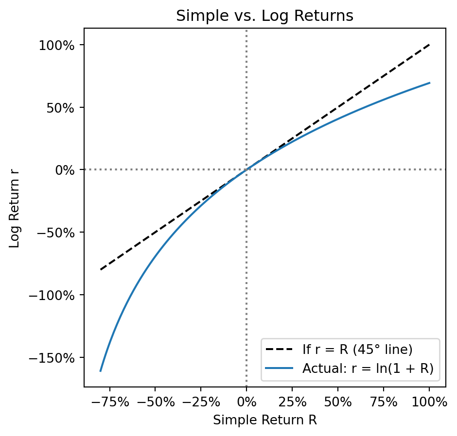
Given a simple return \(R\), what is the equivalent continuously compounded return \(r\)?
By definition, \(r\) is the rate such that continuous compounding gives the same growth:
\[e^r = 1 + R\]
Solving for \(r\):
\[r = \ln(1 + R)\]
This is why they’re called log returns—they’re literally the logarithm of gross returns.
For stocks (ignoring dividends), the gross return is \(1 + R_t = \frac{P_t}{P_{t-1}}\), so:
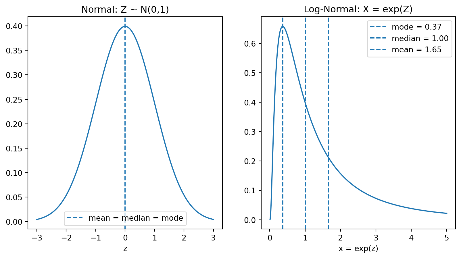
The \(\frac{\sigma^2}{2}\) term is the variance boost. The more spread out \(Z\) is (higher variance), the more the exponential “boosts” the high values relative to the low values.
Expected Wealth After \(T\) Years
Recall: our “naive” forecast for terminal wealth (ignoring variance) was \(W_0 \cdot e^{T\mu}\).
But now we know the true expected value includes the variance boost:
The median is the “typical” outcome. The mean is pulled up by a small number of extremely lucky outcomes—most investors will earn less than the expected value. Let’s simulate this.
import numpy as npimport matplotlib.pyplot as pltfrom scipy import statsnp.random.seed(42)mu, sigma, T =0.0941, 0.1848, 60# Annual log return parametersn_investors =100000W_0 =1# Starting wealth# Step 1: Draw 60 years of log returns for each investor# Each row = one investor, each column = one yearreturns = np.random.normal(mu, sigma, (n_investors, T))print(f"Shape: {returns.shape} (100,000 investors × 60 years)")print(f"First investor's first 5 years: {returns[0, :5].round(3)}")
Shape: (100000, 60) (100,000 investors × 60 years)
First investor's first 5 years: [0.186 0.069 0.214 0.376 0.051]
Each investor gets 60 independent draws from \(N(\mu, \sigma^2)\).
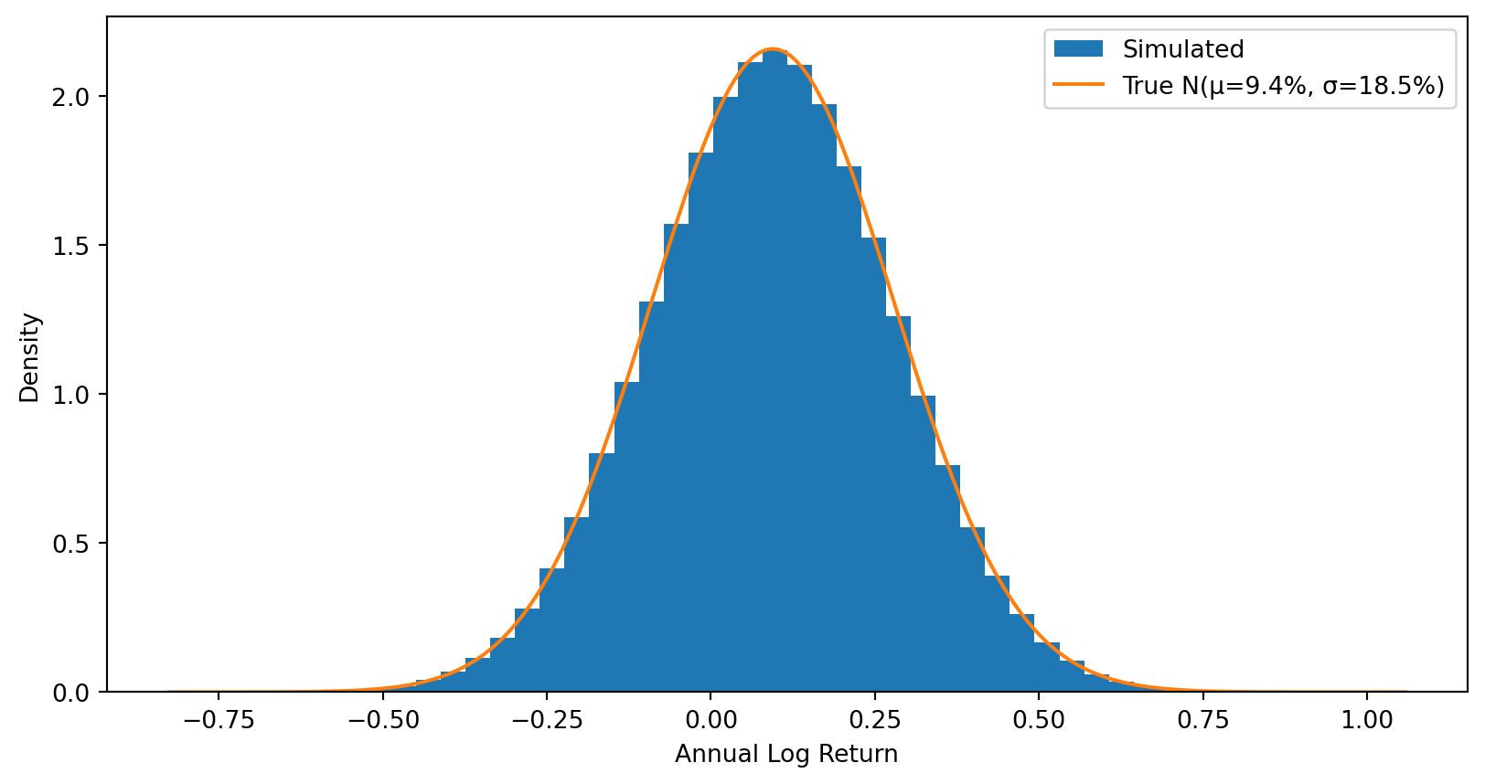
Step 1: Individual annual returns are normally distributed (symmetric).
# The distribution of individual annual returnsall_returns = returns.flatten()plt.hist(all_returns, bins=50, density=True, label='Simulated')# Overlay the true normal distributionx = np.linspace(all_returns.min(), all_returns.max(), 200)plt.plot(x, stats.norm.pdf(x, mu, sigma), label=f'True N(μ={mu:.1%}, σ={sigma:.1%})')plt.xlabel('Annual Log Return')plt.ylabel('Density')plt.legend()plt.show()
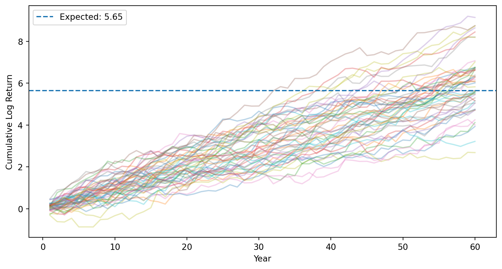
Step 2: Log returns accumulate over time (still symmetric).
# Cumulative log returns (running sum over time)cumulative_log_returns = np.cumsum(returns, axis=1)# Plot sample paths for a few investorsfor i inrange(50): plt.plot(range(1, T+1), cumulative_log_returns[i], alpha=0.3)plt.axhline(mu * T, linestyle='--', label=f'Expected: {mu*T:.2f}')plt.xlabel('Year')plt.ylabel('Cumulative Log Return')plt.legend()plt.show()
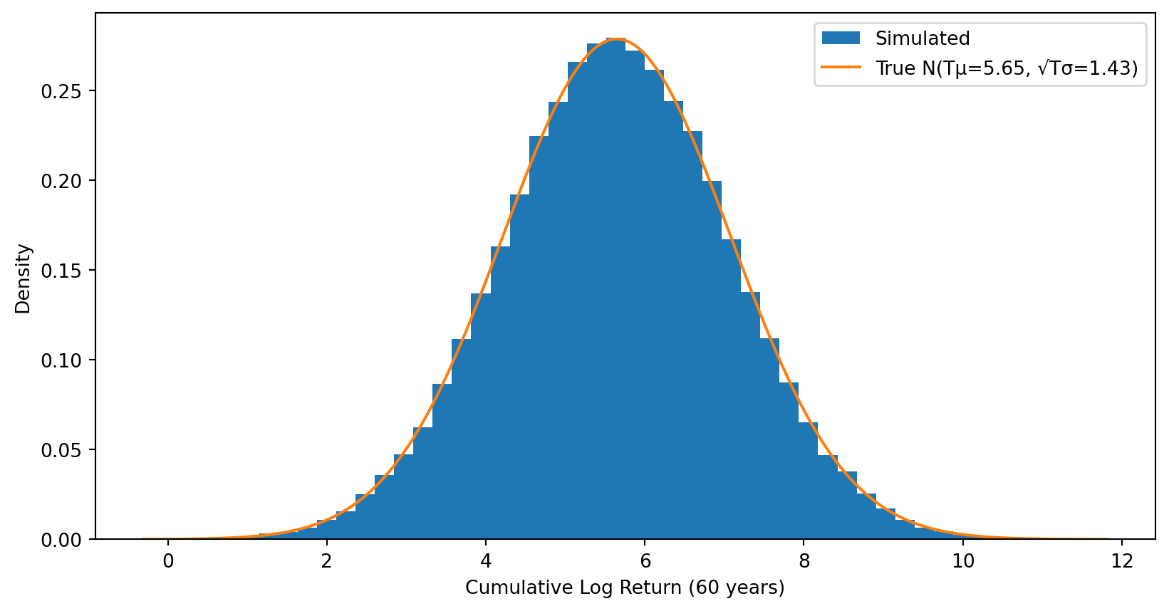
After 60 years, cumulative log return \(\sim N(T\mu, T\sigma^2)\) — still symmetric.
# Distribution of terminal cumulative log returnsterminal_log_returns = cumulative_log_returns[:, -1]plt.hist(terminal_log_returns, bins=50, density=True, label='Simulated')# Overlay the true normal distribution: N(T*mu, T*sigma^2)x = np.linspace(terminal_log_returns.min(), terminal_log_returns.max(), 200)plt.plot(x, stats.norm.pdf(x, mu*T, sigma*np.sqrt(T)), label=f'True N(Tμ={mu*T:.2f}, √Tσ={sigma*np.sqrt(T):.2f})')plt.xlabel('Cumulative Log Return (60 years)')plt.ylabel('Density')plt.legend()plt.show()
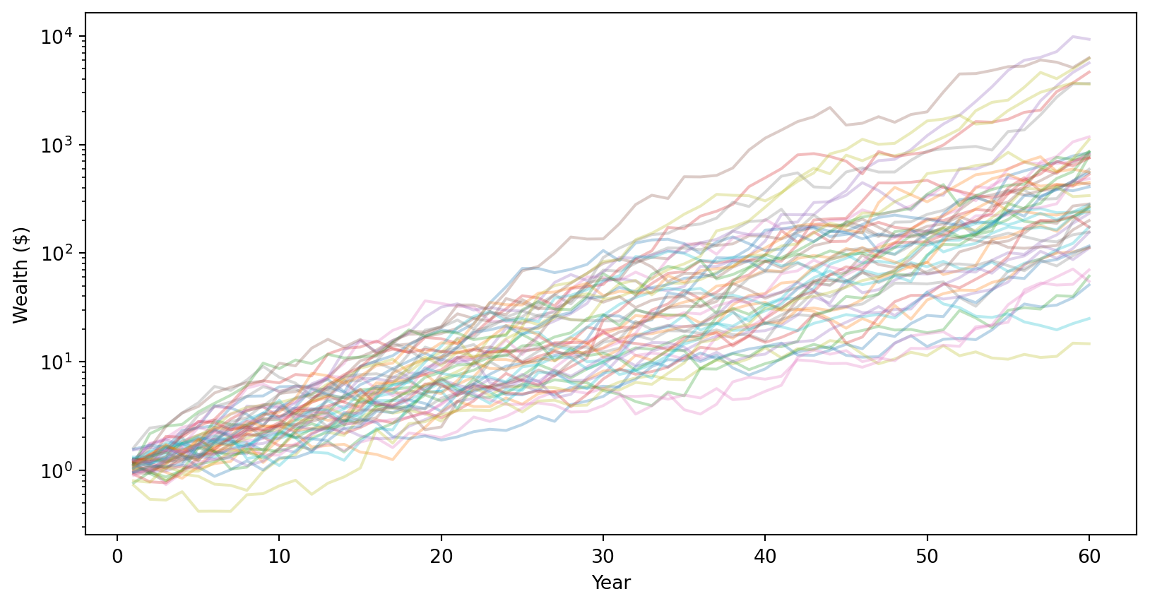
Step 3: Exponentiate to get wealth (now asymmetric!).
# Convert to wealth by exponentiating: W_T = W_0 * exp(cumulative log return)wealth_paths = W_0 * np.exp(cumulative_log_returns)# Plot sample pathsfor i inrange(50): plt.plot(range(1, T+1), wealth_paths[i], alpha=0.3)plt.xlabel('Year')plt.ylabel('Wealth ($)')plt.yscale('log') # Log scale to see all pathsplt.show()
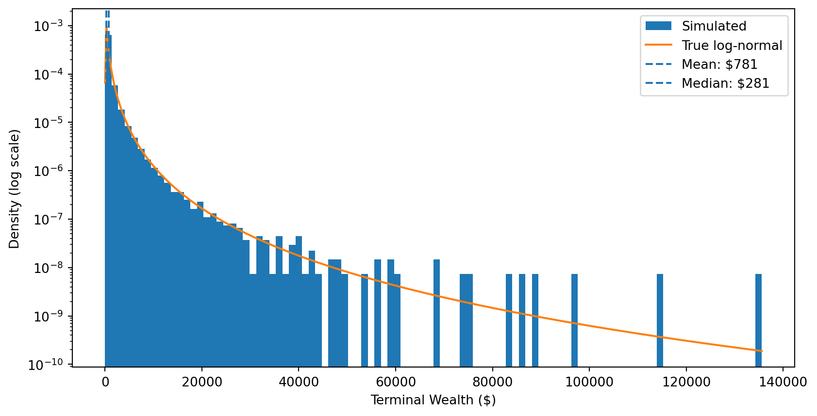
Step 4: Terminal wealth is log-normally distributed.
# Final wealth after 60 yearsterminal_wealth = wealth_paths[:, -1]plt.hist(terminal_wealth, bins=100, density=True, label='Simulated')# Overlay the true log-normal distribution# If ln(W) ~ N(m, v), then W is log-normal with scale=exp(m) and s=sqrt(v)x = np.linspace(terminal_wealth.min(), terminal_wealth.max(), 500)plt.plot(x, stats.lognorm.pdf(x, s=sigma*np.sqrt(T), scale=np.exp(mu*T)), label='True log-normal')plt.axvline(np.mean(terminal_wealth), linestyle='--', label=f'Mean: ${np.mean(terminal_wealth):.0f}')plt.axvline(np.median(terminal_wealth), linestyle='--', label=f'Median: ${np.median(terminal_wealth):.0f}')plt.xlabel('Terminal Wealth ($)')plt.ylabel('Density (log scale)')# plt.xscale('log')plt.yscale('log')plt.legend()plt.show()print(f"{100*np.mean(terminal_wealth < np.mean(terminal_wealth)):.0f}% of investors earn less than the mean!")
76% of investors earn less than the mean!
The punchline: Most investors earn less than the expected value!
The Punchline: Expected Value Is Biased Upward
Summary of Part I:
Log returns assumed normal \(\implies\) wealth is log-normal
The expected value of a log-normal includes a variance boost: \(e^{T\sigma^2/2}\)
This boost grows with time horizon \(T\) and volatility \(\sigma^2\)
As a result: Mean \(>\) Median \(>\) Mode for terminal wealth
The implication:
If you use expected wealth to plan for retirement (or advise clients), you will systematically overestimate what most people will actually experience.
Next: How do we adjust for this bias? And where does the uncertainty come from?
Part II: Estimation Risk
From Known to Unknown Parameters
In Part I, we treated \(\mu\) and \(\sigma^2\) as known parameters.
Reality: We don’t know the true expected return \(\mu\). We must estimate it from historical data.
This introduces estimation risk—additional uncertainty because our parameters are estimates, not truth.
Key question: If we plug our estimate \(\hat{\mu}\) into the wealth formula, do we get an unbiased forecast of expected wealth?
Spoiler: No. There’s an additional source of upward bias beyond what we saw in Part I.
What Is an Unbiased Estimator?
Definition: An estimator \(\hat{\theta}\) is unbiased if its expected value equals the true parameter:
\[\mathbb{E}[\hat{\theta}] = \theta\]
Example: The sample mean \(\bar{r} = \frac{1}{N}\sum_{i=1}^{N} r_i\) is an unbiased estimator of \(\mu\).
Why should we care?
Unbiased estimators are correct on average over repeated sampling
The correction term \(\frac{T^2\sigma^2}{2N}\) removes the upward bias caused by estimation risk.
Reference: This adjustment is derived in Jacquier, Kane, and Marcus (2003), “Geometric or Arithmetic Mean: A Reconsideration,” Financial Analysts Journal.
Intuition: We’re subtracting out the “extra variance” that comes from not knowing \(\mu\) perfectly.
Two Sources of Uncertainty
Our wealth forecast faces two distinct sources of uncertainty:
Return risk: Future returns are random
Variance contribution to \(\ln(W_T)\): \(T\sigma^2\)
Grows linearly with horizon \(T\)
Estimation risk: We don’t know \(\mu\) exactly
Variance contribution to forecast: \(\frac{T^2\sigma^2}{N}\)
Example:\(\sigma = 20\%\), \(N = 100\) years of data
Horizon \(T\)
Return risk
Estimation risk
Ratio
\(T\sigma^2\)
\(\frac{T^2\sigma^2}{N}\)
1 year
0.04
0.0004
1%
10 years
0.40
0.04
10%
30 years
1.20
0.36
30%
60 years
2.40
1.44
60%
At a 60-year horizon, estimation risk is 60% as large as return risk!
Implication: For long-horizon investors (pension funds, endowments, retirement planning), parameter uncertainty is a first-order concern.
Why Is the Mean So Hard to Estimate?
Comparing precision of \(\hat{\mu}\) vs. \(\hat{\sigma}\):
With \(N = 100\) years of annual data:
Standard error of \(\hat{\mu}\): \(\frac{\sigma}{\sqrt{N}} = \frac{0.20}{\sqrt{100}} = 2\%\)
True \(\mu\) is around 8%, so SE is 25% of the parameter
Standard error of \(\hat{\sigma}\): approximately \(\frac{\sigma}{\sqrt{2N}} \approx 1.4\%\)
True \(\sigma\) is around 20%, so SE is 7% of the parameter
The mean is much harder to estimate than volatility.
Volatility is estimated from squared deviations (lots of signal each period). The mean requires averaging returns that are very noisy relative to their expected value.
Summary of Part II
Key takeaways:
While \(\hat{\mu}\) is an unbiased estimator of \(\mu\), the wealth forecast \(\widehat{W}_T\) is not an unbiased estimator of \(\mathbb{E}[W_T]\)
The bias factor is \(\exp\left(\frac{T^2\sigma^2}{2N}\right)\)—it grows with \(T^2\)
We can correct for this bias by subtracting \(\frac{T^2\sigma^2}{2N}\) from the exponent
Estimation risk grows faster than return risk as horizon increases
Practical implication: Be skeptical of long-horizon wealth projections. They compound two sources of upward bias: the log-normal effect (Part I) and estimation error (Part II).
Looking Ahead: Why This Matters for Machine Learning