RSM338: Machine Learning in Finance
Week 9: Ensemble Methods | March 18–19, 2026
Kevin Mott
Rotman School of Management
Today’s Goal
Last week we saw that decision trees are interpretable and flexible, but they have a serious weakness: high variance. Small changes in the training data can produce completely different trees.
Today we fix this by combining many trees into an ensemble—a team of models that’s stronger than any individual.
Today’s roadmap:
- The ensemble idea: Why combining models reduces error
- Random Forests: Many trees, each trained on random subsets of data and features
- Boosting: Trees built sequentially, each correcting the previous one’s mistakes
- XGBoost: Industrial-strength gradient boosting
Recap: Decision Trees and Their Weakness
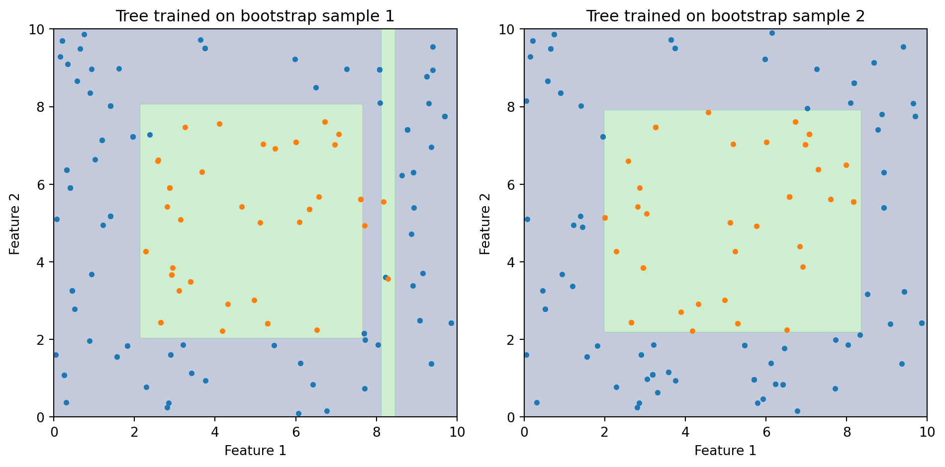
Decision trees partition the feature space using a sequence of yes/no splits. They’re easy to interpret and handle nonlinear relationships—but they’re unstable.
Same underlying data, two different bootstrap samples → two very different decision boundaries. This is what high variance looks like.
Part I: The Ensemble Idea
Wisdom of Crowds
In 1906, Francis Galton observed that when a crowd of 800 people guessed the weight of an ox at a county fair, the average of their guesses was nearly perfect—closer to the true weight than almost any individual guess.
The same principle applies to models. If individual models make errors that are somewhat independent, averaging their predictions cancels out the errors.
One decision tree might overfit to noise in one part of the data, while another tree overfits to different noise. When we combine them, the individual mistakes wash out and what remains is the true signal.
This is the core idea behind ensemble methods: a committee of models outperforms any single member.
Why Averaging Reduces Variance
Suppose we have \(B\) models, each with variance \(\sigma^2\). If the models are independent, the variance of their average is:
\[\text{Var}\left(\frac{1}{B}\sum_{b=1}^{B} f_b(x)\right) = \frac{\sigma^2}{B}\]
With 100 independent models, we cut the variance by a factor of 100. More models = less variance.
In other words: each individual model might be noisy, but the noise averages out when we combine many of them. The signal—which is the same across all models—survives the averaging.
The Independence Problem
The \(\sigma^2 / B\) formula assumes the models are independent. In practice, models trained on the same data are correlated—they tend to make similar mistakes.
When models have pairwise correlation \(\rho\) (the Greek letter “rho,” measuring how similar the models’ predictions are), the variance of their average becomes:
\[\text{Var}\left(\bar{f}\right) = \rho\sigma^2 + \frac{1 - \rho}{B}\sigma^2\]
The first term \(\rho\sigma^2\) doesn’t shrink as we add more models—it’s the irreducible cost of correlation. Only the second term decreases with \(B\).
To get the most benefit from ensembling, we need to make the models as different from each other as possible while keeping each one reasonably accurate.
Three Ways to Make Models Different
How can we train models on the same dataset but make them disagree?
| Strategy | How it works | Method |
|---|---|---|
| Different data | Train each model on a random subset of observations | Bagging |
| Different features | At each split, only consider a random subset of features | Random Forests |
| Sequential correction | Each new model focuses on the mistakes of previous ones | Boosting |
Bagging and Random Forests take the parallel approach: train many models independently, then combine. Boosting takes the sequential approach: build models one at a time, each improving on the last.
Bootstrap Sampling
Bootstrap sampling means drawing \(n\) observations from the training data with replacement. Some observations appear multiple times, others are left out entirely.
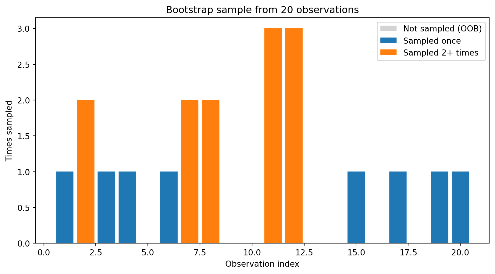
Unique observations in this bootstrap sample: 13 out of 20 (65%)On average, each bootstrap sample contains about 63.2% of the unique observations. The remaining ~36.8% are called out-of-bag (OOB) observations—we’ll use them for free validation later.
Bagging: Bootstrap Aggregation
Bagging (Breiman, 1996) combines bootstrap sampling with model averaging:
- Draw \(B\) bootstrap samples from the training data
- Train one decision tree on each bootstrap sample
- To predict a new observation: have all \(B\) trees vote (classification) or average their predictions (regression)
\[\hat{y}(x) = \text{majority vote of } \{\hat{f}_1(x), \hat{f}_2(x), \ldots, \hat{f}_B(x)\}\]
Each tree sees a slightly different version of the data, so they learn slightly different patterns. The ensemble vote smooths out the individual quirks.
Bagging Visualized
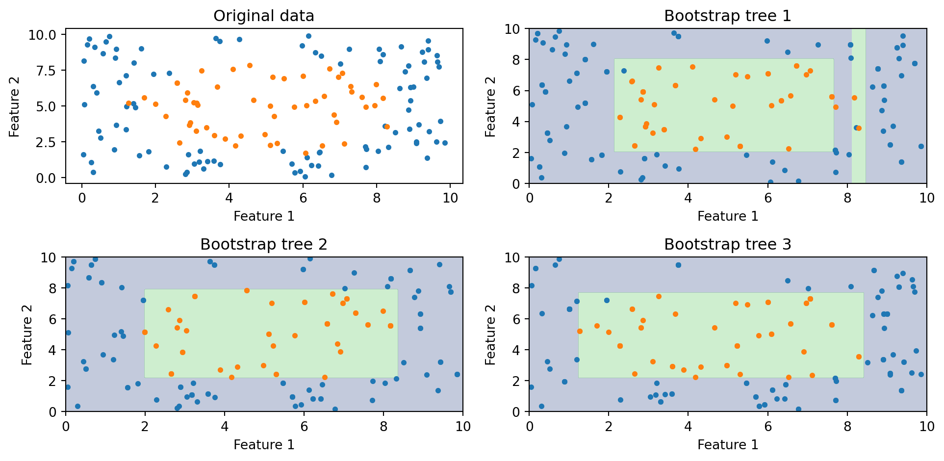
Each bootstrap tree learns a slightly different boundary. When we average all of them, the individual irregularities cancel out and we get a smoother, more stable prediction.
Bagging: What Does It Buy Us?
Bagging reduces variance by averaging over many trees. But there’s a limitation: if one feature is much stronger than the rest, every tree will split on it first. The trees end up highly correlated despite seeing different bootstrap samples.
For example, if FICO score is by far the best predictor of loan default, every bagged tree will put FICO at the root. The trees look similar, \(\rho\) stays high, and the variance reduction is limited.
We need a way to de-correlate the trees further. That’s exactly what Random Forests do.
Part II: Random Forests
Random Forests: Bagging + Feature Subsampling
Random Forests (Breiman, 2001) add one twist to bagging: at each split in each tree, only a random subset of features is considered as candidates.
The algorithm:
- Draw a bootstrap sample
- Grow a tree, but at each split:
- Randomly select \(m_{\text{try}}\) features out of the \(p\) available
- Find the best split among only those \(m_{\text{try}}\) features
- Repeat for \(B\) trees
- Predict by majority vote (classification) or average (regression)
This forces each tree to explore different parts of the feature space, making the trees less correlated with each other.
How Many Features to Consider? (\(m_{\text{try}}\))
\(m_{\text{try}}\) (sometimes written max_features) controls how many features each split is allowed to see. Common defaults:
| Task | Default \(m_{\text{try}}\) | With \(p = 16\) features |
|---|---|---|
| Classification | \(\sqrt{p}\) | 4 features per split |
| Regression | \(p/3\) | ~5 features per split |
Smaller \(m_{\text{try}}\) → trees are more different from each other (lower \(\rho\)), but each individual tree is weaker. Larger \(m_{\text{try}}\) → individual trees are stronger, but they’re more correlated.
When \(m_{\text{try}} = p\), Random Forest reduces to ordinary bagging—every feature is available at every split.
Why Feature Subsampling Helps
Imagine you have 10 features, but FICO score is the strongest predictor. Without feature subsampling:
- Every tree splits on FICO first → high correlation between trees → limited variance reduction
With feature subsampling (\(m_{\text{try}} = 3\)):
- Some trees don’t see FICO at the first split and must use income, DTI, or other features
- These trees discover useful patterns that FICO-dominated trees miss
- Each individual tree may be slightly less accurate, but the ensemble is better
The tradeoff: individual trees get slightly worse, but the reduced correlation makes the ensemble stronger. The whole is greater than the sum of its parts.
Out-of-Bag (OOB) Error Estimation
Each bootstrap sample leaves out some fraction of the training data. For any given observation, we can collect predictions from all the trees that didn’t include it in their bootstrap sample. This gives us a free validation estimate.
OOB error estimation:
- For each training observation \(i\), identify all trees where \(i\) was out-of-bag
- Average (or vote) the predictions from those trees only
- Compare to the true label
- Average across all observations
The OOB error is approximately equivalent to leave-one-out cross-validation, but comes for free—no need for a separate validation set or a cross-validation loop.
Feature Importance in Random Forests
Random Forests provide two measures of which features matter most:
Impurity-based importance (the default in scikit-learn): For each feature, sum up the total reduction in Gini impurity across all splits that use that feature, across all trees. Features that produce larger drops in impurity are ranked as more important.
Permutation importance: Randomly shuffle one feature’s values and measure how much the model’s accuracy drops. If shuffling a feature hurts accuracy a lot, that feature was important. If shuffling barely matters, the feature was dispensable.
Permutation importance is generally more reliable, but impurity-based importance is faster and often gives similar rankings.
Random Forest in Python
from sklearn.ensemble import RandomForestClassifier
from sklearn.datasets import make_classification

# Generate synthetic data
X_synth, y_synth = make_classification(
    n_samples=500, n_features=10, n_informative=5,
    random_state=42
)

# Train a Random Forest
rf = RandomForestClassifier(
    n_estimators=100,      # number of trees
    max_features='sqrt',   # features per split = sqrt(p)
    oob_score=True,        # compute out-of-bag accuracy
    random_state=42
)
rf.fit(X_synth, y_synth)

print(f"OOB accuracy: {rf.oob_score_:.3f}")
print(f"Training accuracy: {rf.score(X_synth, y_synth):.3f}")
OOB accuracy: 0.906
Training accuracy: 1.000The gap between training accuracy and OOB accuracy gives us a sense of how much the model is overfitting. OOB accuracy is a realistic estimate of out-of-sample performance.
Effect of Number of Trees
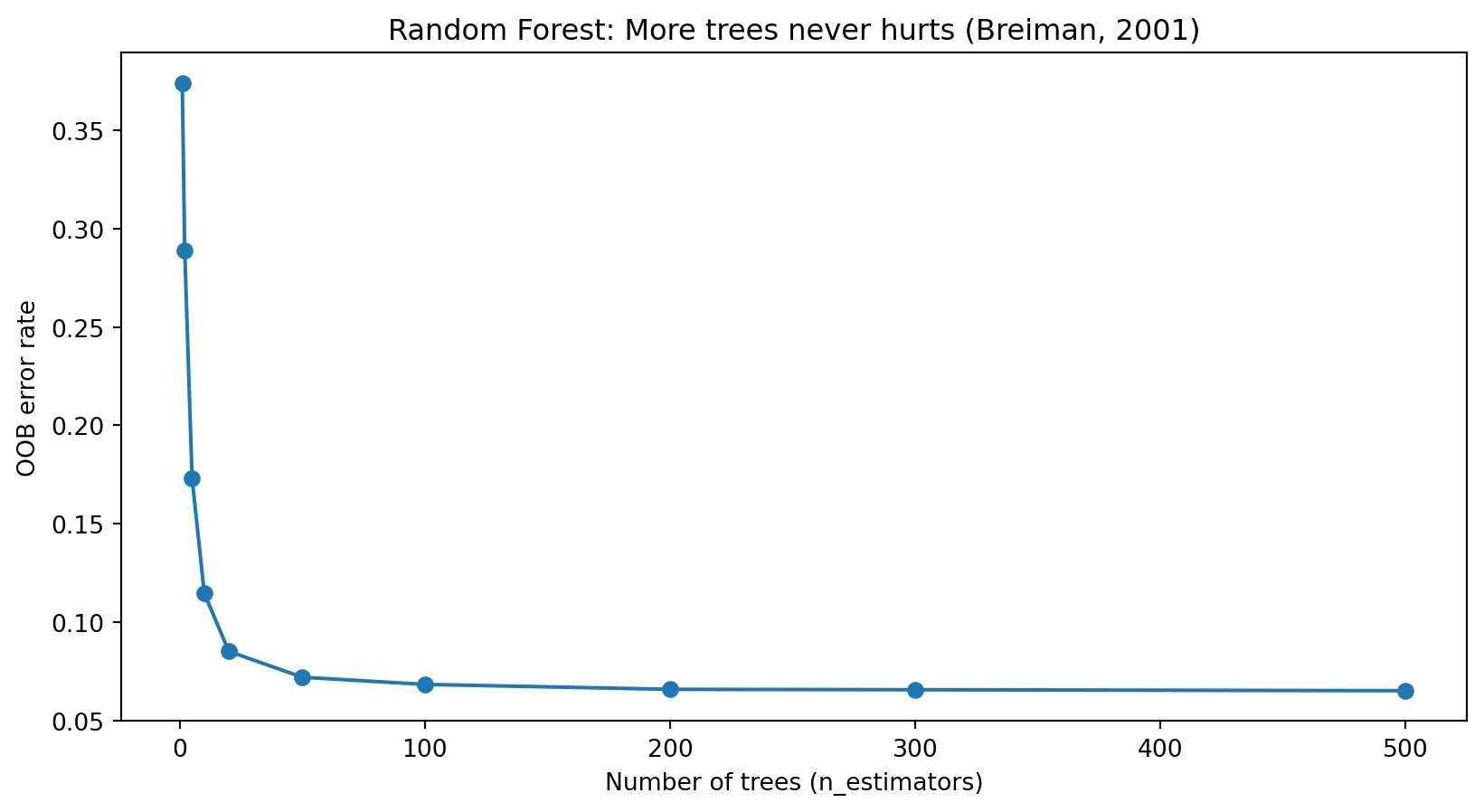
OOB error decreases as we add more trees and eventually levels off. Unlike many models, Random Forests cannot overfit by adding more trees—more trees only means more stable averaging. The main cost is computation time.
Random Forest Hyperparameters
| Parameter | What it controls | Typical range |
|---|---|---|
n_estimators |
Number of trees in the forest | 100–1000 (more is better, but slower) |
max_features |
Features considered per split | 'sqrt' (classification), p/3 (regression) |
max_depth |
Maximum depth of each tree | None (fully grown) or 10–30 |
min_samples_leaf |
Minimum observations in a leaf | 1–10 |
In practice, the default values work well for most problems. The main tuning decision is n_estimators—use as many trees as your computational budget allows.
Random Forest: Averaging Smooths Out Overfitting
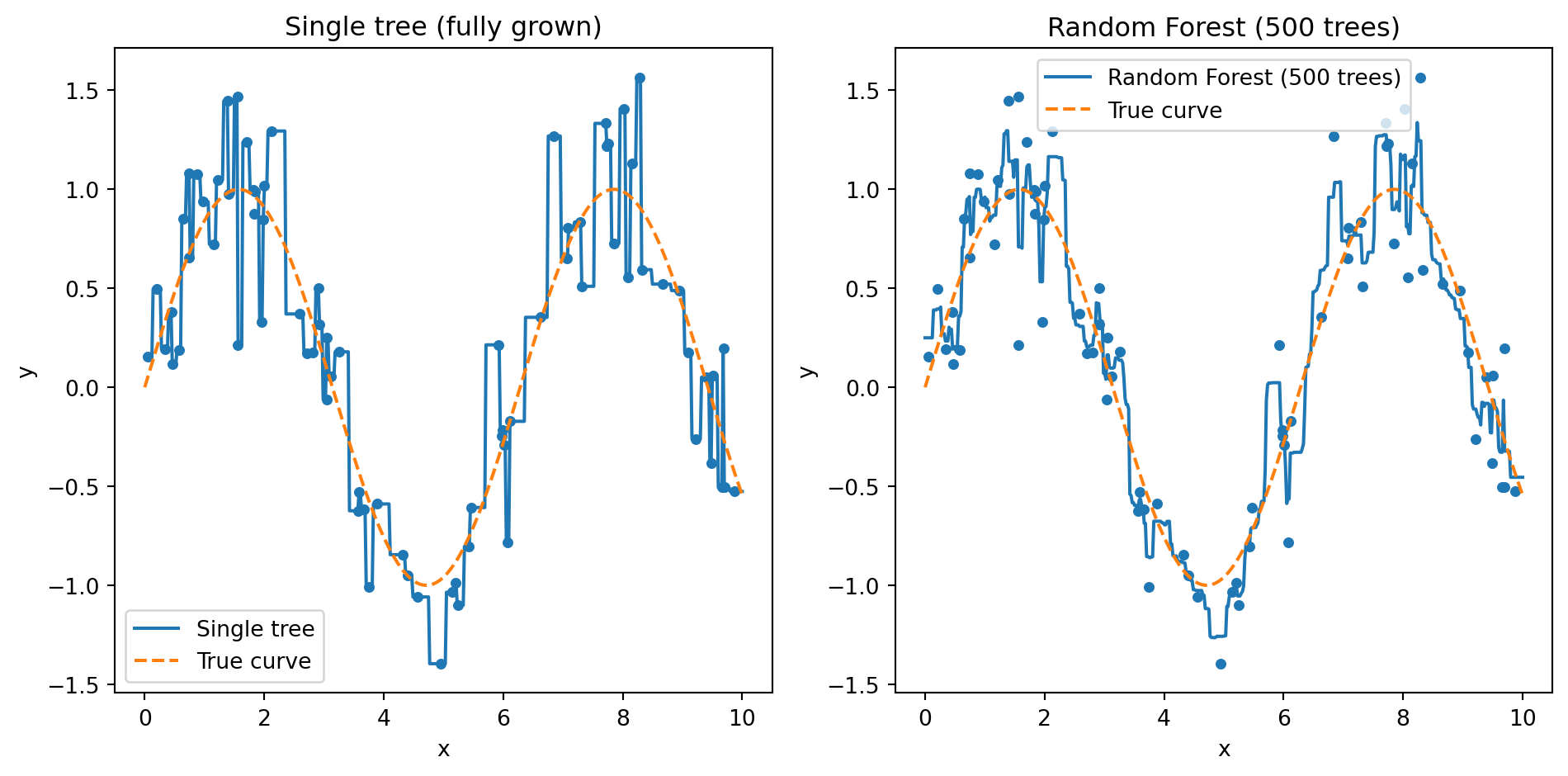
The left panel shows a single fully-grown tree: it memorizes every training point, producing a jagged step function that jumps up and down to hit each observation. The right panel shows what happens when we average 100 such trees together. The individual quirks cancel out and the forest recovers a smooth curve close to the true pattern. This is variance reduction in action — each tree overfits differently, but their average does not.
Part III: Boosting
A Different Strategy: Learn from Mistakes
Random Forests reduce variance by averaging many independent models. Boosting takes a completely different approach: build models sequentially, where each new model focuses on the mistakes made by the previous ones.
Think of it like studying for an exam. After your first practice test, you don’t re-study everything equally—you focus on the questions you got wrong. After the second attempt, you focus on the remaining mistakes. Each round of studying targets your weakest areas.
Boosting does the same thing with models: each new tree pays extra attention to the observations that previous trees got wrong.
Weak Learners
Boosting works with weak learners—models that are only slightly better than random guessing. For classification, “slightly better than random” means accuracy above 50%.
The typical weak learner is a decision stump: a tree with just one split (depth = 1). A stump can only ask one question (“Is FICO > 700?”), so it’s a very limited model on its own.
Schapire (1990) proved a remarkable theoretical result: any combination of weak learners can be boosted into a strong learner with arbitrarily high accuracy. You don’t need good individual models—you just need lots of slightly-better-than-random models that each fix a different part of the problem.
A Note on What Comes Next
We’re now in the “Advanced Topics” part of the course (Weeks 9–11). Up to this point, most methods had natural visual representations — decision boundaries, tree diagrams, variance-reduction plots. From here on, some of the most important algorithms don’t lend themselves to a single clean picture. AdaBoost, for instance, is fundamentally a sequential process of re-weighting and voting — you can plot individual rounds, but the picture doesn’t convey the algorithm the way a decision tree diagram does.
So we’re going to shift gears. Instead of leading with visualizations, we’ll walk through the algorithms step by step — what happens in each round, what the formulas compute, and why. If a picture helps, we’ll use one. But the goal is for you to be able to trace through the algorithm on paper, not just recognize a plot.
AdaBoost: The Idea
AdaBoost (Freund & Schapire, 1997) was the first practical boosting algorithm. Here’s how it works, step by step:
- Start: Give every training observation equal weight \(w_i = 1/n\). Train a decision stump on the data.
- Evaluate: The stump gets some observations wrong. Compute its weighted error rate \(\varepsilon\) — how much total weight falls on misclassified points.
- Vote weight: Give this stump a vote weight \(\alpha\) based on its accuracy. Better stumps get louder votes.
- Re-weight: Increase the weights on misclassified points so the next stump will focus on them. Decrease weights on points we already get right.
- Repeat for \(M\) rounds. Each round adds one stump that targets the mistakes left over from previous rounds.
- Final prediction: Take a weighted vote across all \(M\) stumps.
The result is that many weak models — each barely better than a coin flip — combine into a strong classifier.
The AdaBoost Algorithm
Each observation starts with weight \(w_i = 1/n\). In each round \(m = 1, 2, \ldots, M\):
- Fit a weak learner \(h_m(x)\) on the weighted training data
- Compute weighted error — the total weight on misclassified points: \[\varepsilon_m = \frac{\sum_{i:\, h_m(x_i) \neq y_i} w_i}{\sum_{i=1}^{n} w_i}\]
- Compute this stump’s vote weight (Greek letter “alpha”): \[\alpha_m = \frac{1}{2}\ln\!\left(\frac{1 - \varepsilon_m}{\varepsilon_m}\right)\]
- Update weights — multiply each misclassified observation’s weight by \(e^{\alpha_m}\) and each correct observation’s weight by \(e^{-\alpha_m}\), then renormalize so weights sum to 1
Final prediction: AdaBoost is formulated for binary classification where the class labels are coded as \(y_i \in \{-1, +1\}\). Each stump \(h_m(x)\) also outputs \(-1\) or \(+1\), so the weighted sum \(\sum \alpha_m h_m(x)\) is positive when the \(+1\) votes outweigh the \(-1\) votes and negative otherwise. The \(\text{sign}\) function simply reads off which class won:
\[\hat{y}(x) = \text{sign}\!\left(\sum_{m=1}^{M} \alpha_m \, h_m(x)\right)\]
Bagging vs. Boosting
| Bagging / Random Forest | Boosting | |
|---|---|---|
| Training | Parallel (trees are independent) | Sequential (each tree depends on previous) |
| Tree type | Full-sized, deep trees | Shallow trees (weak learners) |
| Primary benefit | Reduces variance | Reduces bias (and variance) |
| Overfitting risk | Low (more trees never hurts) | Higher (can overfit if too many rounds) |
| Sensitivity to noise | Robust | More sensitive |
| Computation | Easy to parallelize | Harder to parallelize |
Random Forests start with strong individual models and reduce their variance by averaging. Boosting starts with weak models and gradually builds them into a strong model by correcting errors.
From AdaBoost to Gradient Boosting
AdaBoost works by re-weighting misclassified observations. Gradient Boosting (Friedman, 2001) generalized this idea: instead of re-weighting, fit each new tree to the residuals (errors) of the current model.
The intuition is the same—focus on what the model gets wrong—but gradient boosting works with any loss function, not just classification error. This makes it more flexible and more powerful.
The name comes from a connection to gradient descent: each new tree takes a step in the direction that reduces the loss function most.
Gradient Descent Reminder (Week 5)
Recall from our optimization lecture: gradient descent updates parameters by moving in the direction that reduces the loss:
\[\theta_{t+1} = \theta_t - \eta \, \nabla L(\theta_t)\]
where \(\eta\) (Greek letter “eta”) is the learning rate and \(\nabla L\) is the gradient of the loss function—the direction of steepest ascent.
Gradient boosting applies this same idea, but instead of updating numerical parameters, we update our prediction by adding trees one at a time. Let \(F_m(x)\) be the ensemble’s prediction after \(m\) rounds — a running total of every tree’s contribution so far. And let \(h_m(x)\) be the single new tree fit in round \(m\) — the next correction. The update rule is:
\[F_m(x) = F_{m-1}(x) + \eta \cdot h_m(x)\]
Take yesterday’s prediction, and nudge it by a shrunken version of today’s new tree. Each \(h_m\) is chosen to point in the direction that reduces the loss.
Part IV: Gradient Boosting and XGBoost
The Gradient Boosting Algorithm
Input: Training data, a loss function \(L\), number of rounds \(M\), learning rate \(\eta\).
Algorithm:
Start with a constant prediction: \(F_0(x) = \arg\min_c \sum_{i=1}^n L(y_i, c)\)
For \(m = 1, 2, \ldots, M\):
Compute pseudo-residuals for each observation—how far off the current model is: \[r_{im} = -\frac{\partial L(y_i, F_{m-1}(x_i))}{\partial F_{m-1}(x_i)}\]
Fit a small tree \(h_m\) to the pseudo-residuals \(\{(x_i, r_{im})\}\)
Update the model: \[F_m(x) = F_{m-1}(x) + \eta \cdot h_m(x)\]
For squared-error loss, the pseudo-residuals are simply \(r_{im} = y_i - F_{m-1}(x_i)\)—the ordinary residuals. Each new tree literally predicts what the current model is getting wrong. When the pseudo-residuals hit zero, the negative gradient of the loss is zero — the same condition as being at a minimum in ordinary calculus. There is no direction to move that would reduce the loss further, and the algorithm has converged.
Why Shallow Trees?
In Random Forests, each tree is grown deep—the individual trees need to be strong because we’re just averaging them.
In gradient boosting, the strategy is the opposite: each tree should be shallow (typically depth 3–6). Why?
- Each tree is making a small correction to the current model, not trying to solve the whole problem
- Deep trees can overfit the residuals, especially in later rounds when the residuals are small
- Small trees are weak learners—exactly what boosting theory requires
This is a common source of confusion. Random Forests want each tree to be as good as possible. Gradient boosting wants each tree to be a small, cautious correction.
The Learning Rate
The learning rate \(\eta\) controls how much each tree contributes. Smaller \(\eta\) means each tree makes a smaller correction.
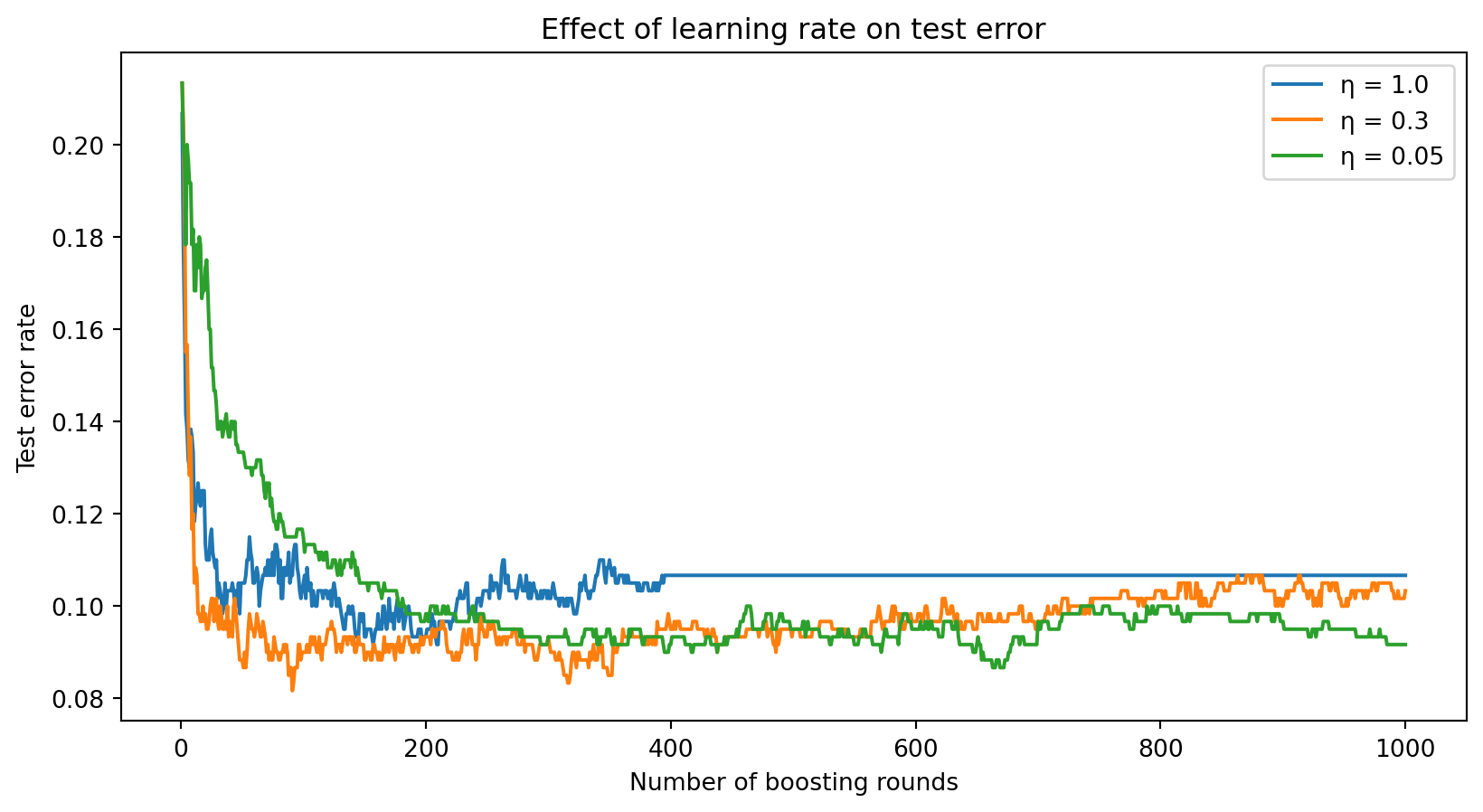
A large learning rate (\(\eta = 1.0\)) converges fast but may overshoot and overfit. A small learning rate (\(\eta = 0.05\)) requires more rounds but often reaches a lower error. The general rule: small \(\eta\) + many trees > large \(\eta\) + few trees.
Gradient Boosting in Python
from sklearn.ensemble import GradientBoostingClassifier
from sklearn.datasets import make_classification
from sklearn.model_selection import train_test_split

# Generate data
X_gb, y_gb = make_classification(
    n_samples=500, n_features=10, n_informative=5,
    random_state=42
)
X_gb_train, X_gb_test, y_gb_train, y_gb_test = train_test_split(
    X_gb, y_gb, test_size=0.3, random_state=42
)

# Train Gradient Boosting
gb = GradientBoostingClassifier(
    n_estimators=200,      # number of boosting rounds
    learning_rate=0.1,     # step size
    max_depth=3,           # shallow trees
    random_state=42
)
gb.fit(X_gb_train, y_gb_train)

print(f"Training accuracy: {gb.score(X_gb_train, y_gb_train):.3f}")
print(f"Test accuracy: {gb.score(X_gb_test, y_gb_test):.3f}")
Training accuracy: 1.000
Test accuracy: 0.920XGBoost: Extreme Gradient Boosting
XGBoost (Chen & Guestrin, 2016) is an optimized implementation of gradient boosting that adds several improvements:
- Regularization: Penalizes complex trees to prevent overfitting
- Efficient computation: Parallelized tree construction, cache-aware design
- Handling missing values: Learns the best direction to send missing values at each split
- Column subsampling: Borrows the Random Forest idea of using random feature subsets (further reduces correlation between trees)
XGBoost became famous through machine learning competitions—it won or placed highly in the majority of structured/tabular data competitions on Kaggle for years. It remains one of the strongest off-the-shelf models for tabular financial data.
XGBoost Objective Function
XGBoost minimizes a regularized objective at each boosting round:
\[\mathcal{L} = \sum_{i=1}^{n} l\!\left(y_i,\; \hat{y}_i + h_m(x_i)\right) + \Omega(h_m)\]
The first term is the usual loss (how well the new tree corrects errors). The second term \(\Omega\) (Greek capital letter “omega”) is a regularization penalty on the tree’s complexity:
\[\Omega(h_m) = \gamma T + \frac{1}{2}\lambda \sum_{j=1}^{T} w_j^2\]
where:
- \(T\) = number of leaves in the tree
- \(w_j\) = prediction value in leaf \(j\)
- \(\gamma\) (gamma) = penalty for adding more leaves (encourages simpler trees)
- \(\lambda\) (lambda) = penalty on leaf weights (prevents extreme predictions)
The regularization is what distinguishes XGBoost from plain gradient boosting. It explicitly trades off prediction accuracy against model complexity.
XGBoost in Python
from xgboost import XGBClassifier
from sklearn.datasets import make_classification
from sklearn.model_selection import train_test_split

# Same data as before
X_xgb, y_xgb = make_classification(
    n_samples=500, n_features=10, n_informative=5,
    random_state=42
)
X_xgb_train, X_xgb_test, y_xgb_train, y_xgb_test = train_test_split(
    X_xgb, y_xgb, test_size=0.3, random_state=42
)

# Train XGBoost
xgb = XGBClassifier(
    n_estimators=200,
    learning_rate=0.1,
    max_depth=3,
    reg_lambda=1.0,        # L2 regularization
    random_state=42
)
xgb.fit(X_xgb_train, y_xgb_train)

print(f"Training accuracy: {xgb.score(X_xgb_train, y_xgb_train):.3f}")
print(f"Test accuracy: {xgb.score(X_xgb_test, y_xgb_test):.3f}")
Training accuracy: 1.000
Test accuracy: 0.920XGBoost Hyperparameters
| Parameter | What it controls | Typical range |
|---|---|---|
n_estimators |
Number of boosting rounds | 100–1000 |
learning_rate |
Step size per round (\(\eta\)) | 0.01–0.3 |
max_depth |
Depth of each tree | 3–8 |
reg_lambda |
L2 regularization on leaf weights (\(\lambda\)) | 0–10 |
subsample |
Fraction of observations per tree | 0.5–1.0 |
colsample_bytree |
Fraction of features per tree | 0.5–1.0 |
subsample and colsample_bytree borrow ideas from bagging and Random Forests—randomly omitting observations and features adds noise that helps prevent overfitting.
Random Forest vs. Gradient Boosting: When to Use Which?
Random Forest:
- A safe default that’s hard to get wrong
- Robust to hyperparameter choices—defaults usually work well
- Easy to parallelize across cores
- Less prone to overfitting
Gradient Boosting / XGBoost:
- Higher ceiling with careful tuning
- Often wins competitions and benchmarks on tabular data
- Requires more hyperparameter tuning (learning rate, depth, regularization)
- Can overfit if not regularized properly
In practice: start with a Random Forest to get a solid baseline. If you need better performance and have time to tune, try XGBoost.
Summary and Preview
What We Learned Today
The ensemble idea: Combining many models reduces error. Averaging independent predictions cuts variance; the key is making models as different as possible.
Random Forests (parallel approach):
- Bagging + random feature subsampling at each split
- Reduces variance by de-correlating trees
- More trees never hurts; robust default hyperparameters
- Free validation via OOB error
Gradient Boosting / XGBoost (sequential approach):
- Each tree corrects the residuals of the previous model
- Reduces bias (and variance through regularization)
- Shallow trees + small learning rate + many rounds
- XGBoost adds regularization and computational efficiency
Next Week: Neural Networks
Ensemble methods excel on structured, tabular data—the kind of data that comes in rows and columns (financial statements, loan applications, trading signals).
But some data isn’t tabular: images, text, audio, time series. These require a different paradigm.
Week 10: Neural Networks
- How neural networks learn nonlinear representations
- Multi-layer perceptrons and backpropagation
- Applications to financial text and image data
References
- Breiman, L. (1996). Bagging predictors. Machine Learning, 24(2), 123–140.
- Breiman, L. (2001). Random forests. Machine Learning, 45(1), 5–32.
- Chen, T. & Guestrin, C. (2016). XGBoost: A scalable tree boosting system. Proceedings of KDD, 785–794.
- Freund, Y. & Schapire, R. E. (1997). A decision-theoretic generalization of on-line learning and an application to boosting. Journal of Computer and System Sciences, 55(1), 119–139.
- Friedman, J. H. (2001). Greedy function approximation: A gradient boosting machine. Annals of Statistics, 29(5), 1189–1232.
- Hastie, T., Tibshirani, R., & Friedman, J. (2009). The Elements of Statistical Learning (2nd ed.). Springer.