Week 8: Nonlinear Classification | March 11–12, 2026
Kevin Mott
Rotman School of Management
Today’s Goal
Last week we learned about linear classification: LDA and logistic regression. These methods assume the decision boundary between classes is a straight line (or hyperplane).
The problem: In many real-world applications, the boundary between classes isn’t linear. Linear classifiers will struggle.
Today’s roadmap:
Why linear fails: When classes aren’t linearly separable
k-Nearest Neighbors: Let the data speak—classify based on similar observations
Decision Trees: Partition the feature space with simple rules
Information Gain: How trees decide where to split
Application: Predicting loan defaults with the Lending Club dataset
Recap: Linear Classification
In Week 7, we saw that linear classifiers make predictions using:
The decision boundary is where \(z(\mathbf{x}) = 0\)—a straight line in 2D, a plane in 3D, a hyperplane in higher dimensions.
Logistic regression transforms this into a probability using the sigmoid function, but the boundary is still linear.
When Linear Classification Works
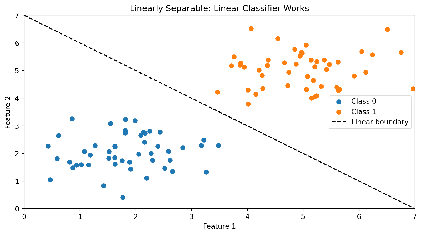
Linear classifiers work well when classes are linearly separable—you can draw a straight line between them.
A simple linear boundary perfectly separates the two classes.
The Feature Engineering Problem
Last week we saw that logistic regression can handle nonlinear boundaries if we add the right transformed features (e.g., \(x_1^2\), \(x_1 x_2\)). The model stays linear in its parameters — we just give it richer inputs.
But that approach has a big limitation: we have to know which transformations to use. With 2 features, adding squares and interactions is easy. With 50 features? There are 1,275 pairwise interactions and 50 squared terms — and we have no guarantee that quadratic terms are the right choice. Maybe the boundary depends on \(\log(x_3)\), or \(x_7 / x_{12}\), or something we’d never think to try.
We want methods that can learn nonlinear boundaries directly from the data, without us having to guess the right feature transformations in advance.
Classification in Finance: The Credit Default Problem
Consider a bank deciding whether to approve a loan. The outcome is binary:
Class 1 (Default): The borrower fails to repay
Class 0 (Repaid): The borrower repays in full
Based on features like credit score, income, and debt-to-income ratio, can we predict who will default?
The relationship between features and default is rarely linear. A borrower with moderate income and moderate credit score might default, while someone with either very high income OR very high credit score might not—this creates complex, non-linear boundaries.
Today we’ll learn two nonparametric methods that can capture these nonlinear patterns: k-Nearest Neighbors and Decision Trees.
Parametric vs. Nonparametric Models
Parametric models (like logistic regression) assume the data follows a specific functional form. We estimate a fixed set of parameters (\(w_0, w_1, \ldots, w_p\)), and these parameters define the model completely.
Nonparametric models make fewer assumptions about the functional form. Instead, they let the data determine the structure of the decision boundary.
Parametric
Nonparametric
Structure
Fixed form (e.g., linear)
Flexible, data-driven
Parameters
Fixed number
Grows with data
Examples
Logistic regression, LDA
k-NN, Decision Trees
Risk
Bias if form is wrong
Overfitting with limited data
Both k-NN and decision trees are nonparametric—they don’t assume a linear (or any particular) decision boundary.
Part I: k-Nearest Neighbors
The Intuition Behind k-NN
k-Nearest Neighbors (k-NN) is based on a simple idea: similar observations should have similar outcomes.
To classify a new observation:
Find the \(k\) training observations closest to it
Take a vote among those \(k\) neighbors
Assign the majority class
If you want to know if a new loan applicant will default, look at applicants in the training data who are most similar to them. If most of those similar applicants defaulted, predict default.
No training phase is needed—k-NN stores all the training data and does the work at prediction time. This is sometimes called a “lazy learner.”
Distance Recap (Week 4)
k-NN needs to measure how far apart two observations are. Same idea as clustering:
Standardize first. Features on different scales (income in dollars vs. DTI as a ratio) will make distance meaningless. Standardize each feature to mean 0, standard deviation 1.
Distance = norm of a difference. The \(L_2\) (Euclidean) norm is the default. Manhattan (\(L_1\)) is an alternative but Euclidean works well for most applications.
The k-NN Algorithm
Input: Training data \(\{(\mathbf{x}_1, y_1), \ldots, (\mathbf{x}_n, y_n)\}\), a new point \(\mathbf{x}\), and the number of neighbors \(k\).
Algorithm:
Compute the distance from \(\mathbf{x}\) to every training observation \(\mathbf{x}_i\)
Identify the \(k\) training observations with the smallest distances—call this set \(\mathcal{N}_k(\mathbf{x})\)
Assign the class that appears most frequently among the \(k\) neighbors:
The notation \(\unicode{x1D7D9}_{\{y_i = c\}}\) is the indicator function: it equals 1 if \(y_i = c\) and 0 otherwise. So we’re just counting votes.
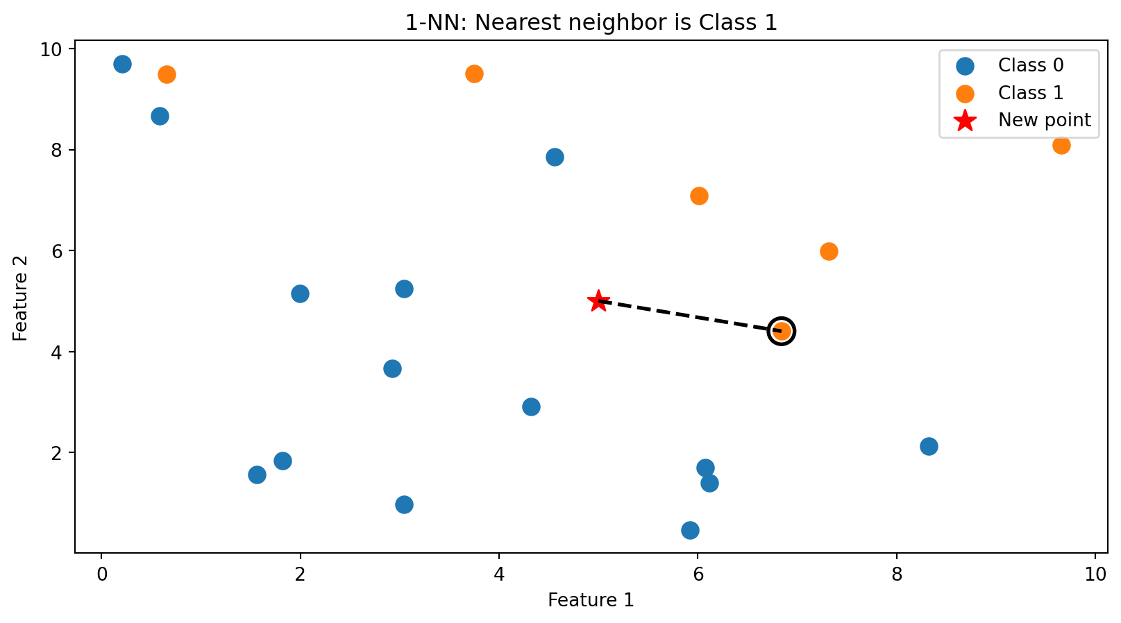
k-NN in Action: k = 1
With \(k = 1\), we classify based on the single closest training point. The new point (star) is assigned the class of its nearest neighbor (circled).
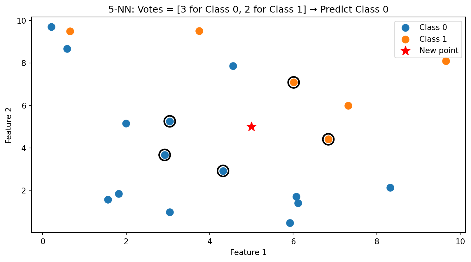
k-NN in Action: k = 5
With \(k = 5\), we take a majority vote among the 5 nearest neighbors (circled). This is more robust than using just one neighbor.
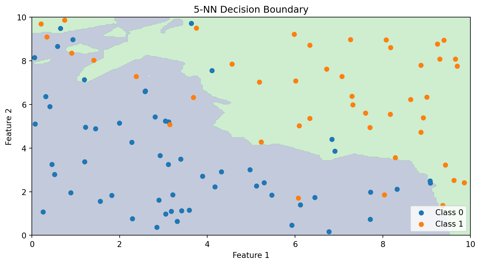
The Decision Boundary of k-NN
Unlike linear classifiers, k-NN doesn’t explicitly compute a decision boundary. But we can visualize what the boundary looks like by classifying every point in the feature space.
The k-NN decision boundary is nonlinear and adapts to the local density of data. It naturally forms complex shapes without us specifying any functional form.
The Role of k: Bias-Variance Tradeoff
The choice of \(k\) is crucial:
Small k (e.g., k = 1):
Boundary closely follows the training data
Very flexible—can capture complex patterns
High variance, low bias
Risk of overfitting (sensitive to noise)
Large k (e.g., k = 100):
Boundary is smoother
Less flexible—averages over many neighbors
Low variance, high bias
Risk of underfitting (misses local patterns)
This is the bias-variance tradeoff we’ve seen before. We need to choose \(k\) that balances these concerns.
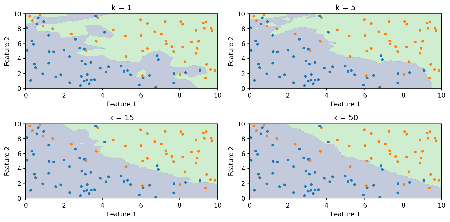
Effect of k on the Decision Boundary
As \(k\) increases, the boundary becomes smoother. With \(k = 1\), every training point gets its own region. With large \(k\), the boundary approaches the overall majority class.
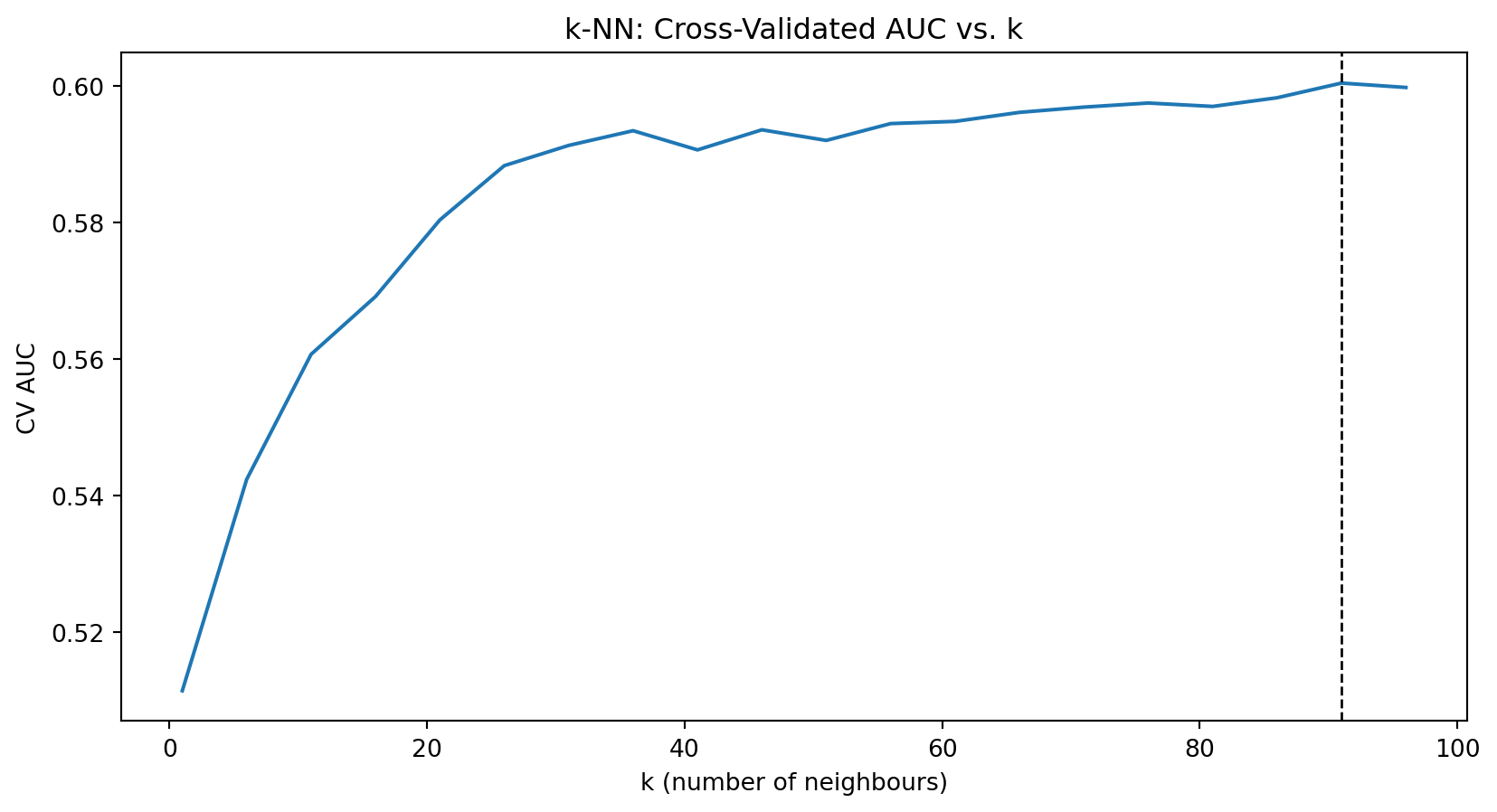
Choosing k with Cross-Validation
How do we choose \(k\)? Use cross-validation (from Week 5):
Split training data into folds
For each candidate value of \(k\):
Fit k-NN on training folds
Evaluate accuracy on validation fold
Choose \(k\) that maximizes cross-validated accuracy
A common rule of thumb: \(k < \sqrt{n}\) where \(n\) is the sample size. But cross-validation is more reliable.
from sklearn.neighbors import KNeighborsClassifierfrom sklearn.model_selection import cross_val_scoreimport numpy as np# Try different values of kk_values =range(1, 31)cv_scores = []for k in k_values: knn = KNeighborsClassifier(n_neighbors=k) scores = cross_val_score(knn, X_train, y_train, cv=5) cv_scores.append(scores.mean())best_k = k_values[np.argmax(cv_scores)]print(f"Best k: {best_k} with CV accuracy: {max(cv_scores):.3f}")
Best k: 19 with CV accuracy: 0.850
k-NN: Advantages and Disadvantages
Advantages:
Simple to understand and implement
No training phase (just store the data)
Naturally handles multi-class problems
Can capture complex, nonlinear boundaries
No assumptions about the data distribution
Disadvantages:
Slow at prediction time—must compute distances to all training points
Doesn’t work well in high dimensions (“curse of dimensionality”)
Sensitive to irrelevant features (all features contribute to distance)
Requires feature scaling
For large datasets, approximate nearest neighbor methods can speed up k-NN, but it remains computationally intensive.
The Curse of Dimensionality
k-NN relies on distance, and distance breaks down in high dimensions. Three related problems:
The space becomes sparse. In 1D, 100 points cover the range well. In 2D, the same 100 points are scattered across a plane. In 50D, they’re lost in a vast empty space. The amount of data you need to “fill” the space grows exponentially with \(p\).
You need more data to have local neighbours. If the space is mostly empty, the \(k\) “nearest” neighbours may be far away — and far-away neighbours aren’t informative about the local structure.
Distances become less informative. Euclidean distance sums \(p\) squared differences. As \(p\) grows, all these sums converge to roughly the same value (law of large numbers). The nearest and farthest neighbours end up almost the same distance away, so “nearest” stops meaning much.
Part II: Decision Trees
The Intuition Behind Decision Trees
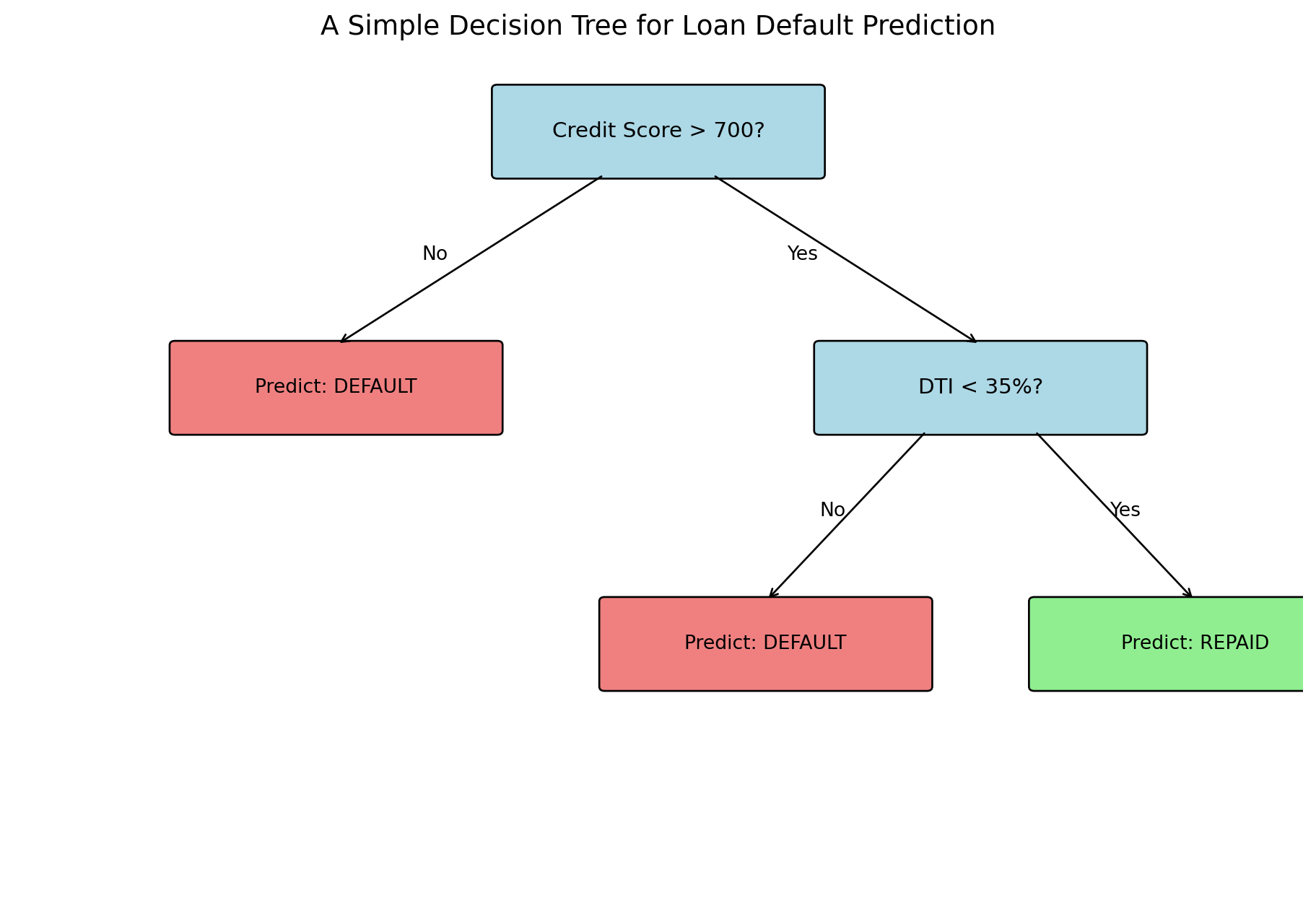
Decision trees mimic how humans make decisions: a series of yes/no questions.
Consider a loan officer evaluating an application:
Is the credit score above 700?
If no → High risk, deny
If yes → Continue…
Is the debt-to-income ratio below 35%?
If no → Medium risk, deny
If yes → Low risk, approve
Each question splits the population into subgroups, and we make predictions based on which group an observation falls into.
Decision trees automate this process: they learn which questions to ask and in what order.
Anatomy of a Decision Tree
Terminology:
Root node: The first split (top of the tree)
Internal nodes: Decision points that split the data
Leaf nodes: Terminal nodes that make predictions
Depth: The number of splits from root to leaf
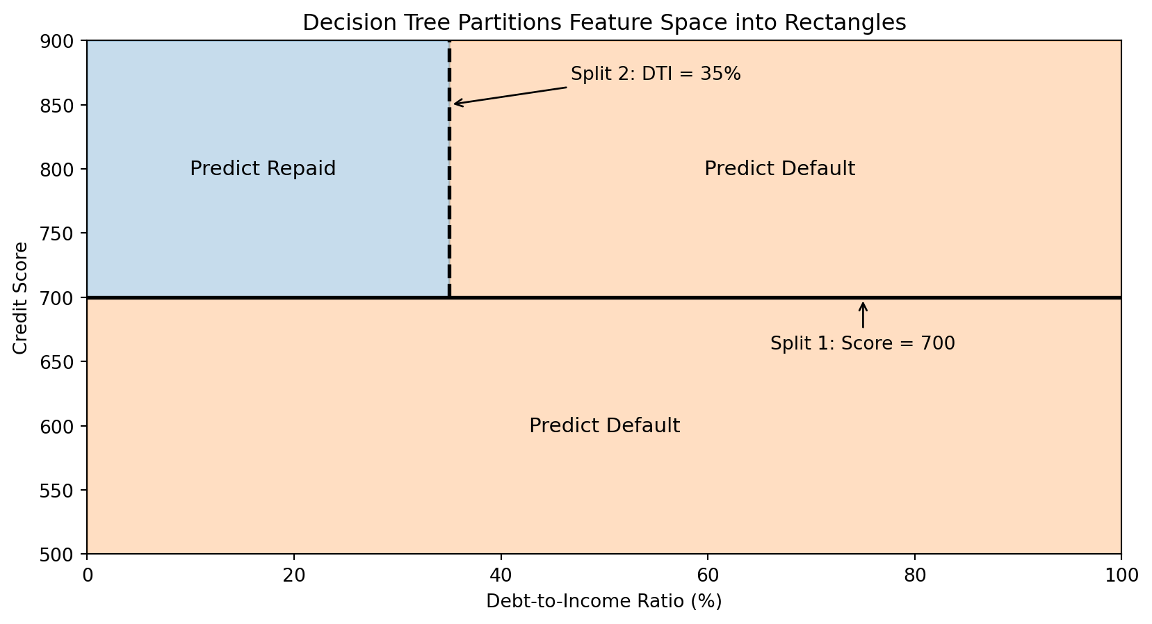
How Trees Partition the Feature Space
Each split in a decision tree divides the feature space with an axis-aligned boundary (parallel to one axis).
The tree creates rectangular regions. Each leaf corresponds to one region, and all observations in that region get the same prediction.
The Decision Tree Algorithm: Recursive Partitioning
The Goal: Build a tree that makes good predictions.
The Approach: Greedy, recursive partitioning.
Start with all training data at the root
Find the best split—the feature and threshold that best separates the classes
Split the data into two groups based on this rule
Recursively apply steps 2-3 to each group
Stop when a stopping criterion is met (e.g., minimum samples per leaf, maximum depth)
The key question: How do we define “best” split?
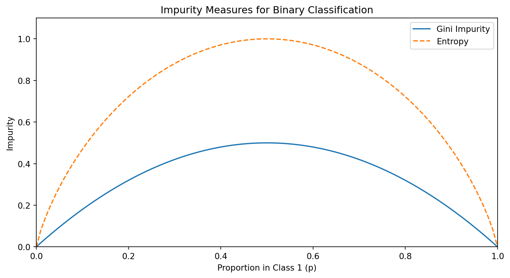
Measuring Split Quality: Impurity
A good split should create child nodes that are more “pure” than the parent—ideally, each child contains only one class.
We measure impurity—how mixed the classes are in a node. A pure node (all one class) has impurity = 0.
For a node with \(n\) observations where \(p_c\) is the proportion belonging to class \(c\):
We’d compute this for all possible features and thresholds, then choose the split with highest gain.
For Continuous Features: Finding the Best Threshold
For a continuous feature (like credit score), we need to find the best threshold for splitting.
Algorithm:
Sort the observations by the feature value
Consider each unique value as a potential threshold
For each threshold, compute the information gain
Choose the threshold with the highest gain
If there are \(n\) unique values, we evaluate up to \(n-1\) possible splits for that feature. This is computationally tractable because we can update class counts incrementally as we move through sorted values.
Building a Tree in Python
from sklearn.tree import DecisionTreeClassifierimport numpy as np# Generate sample datanp.random.seed(42)n =200credit_score = np.random.normal(700, 50, n)dti = np.random.normal(30, 10, n)X = np.column_stack([credit_score, dti])# Default probability depends on both featuresprob_default =1/ (1+ np.exp(0.02* (credit_score -680) -0.05* (dti -35)))y = (np.random.random(n) < prob_default).astype(int)# Fit decision treetree = DecisionTreeClassifier(max_depth=3, random_state=42)tree.fit(X, y)print(f"Tree depth: {tree.get_depth()}")print(f"Number of leaves: {tree.get_n_leaves()}")print(f"Training accuracy: {tree.score(X, y):.3f}")
Tree depth: 3
Number of leaves: 8
Training accuracy: 0.720
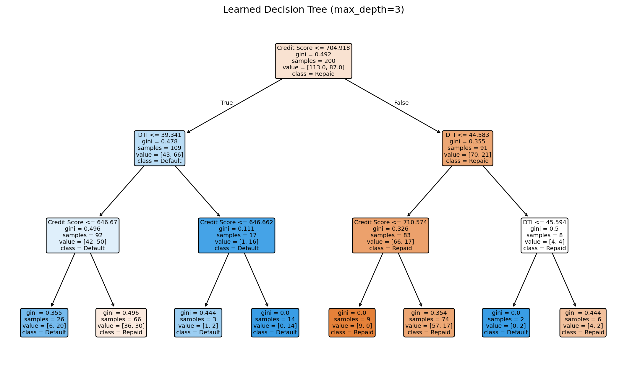
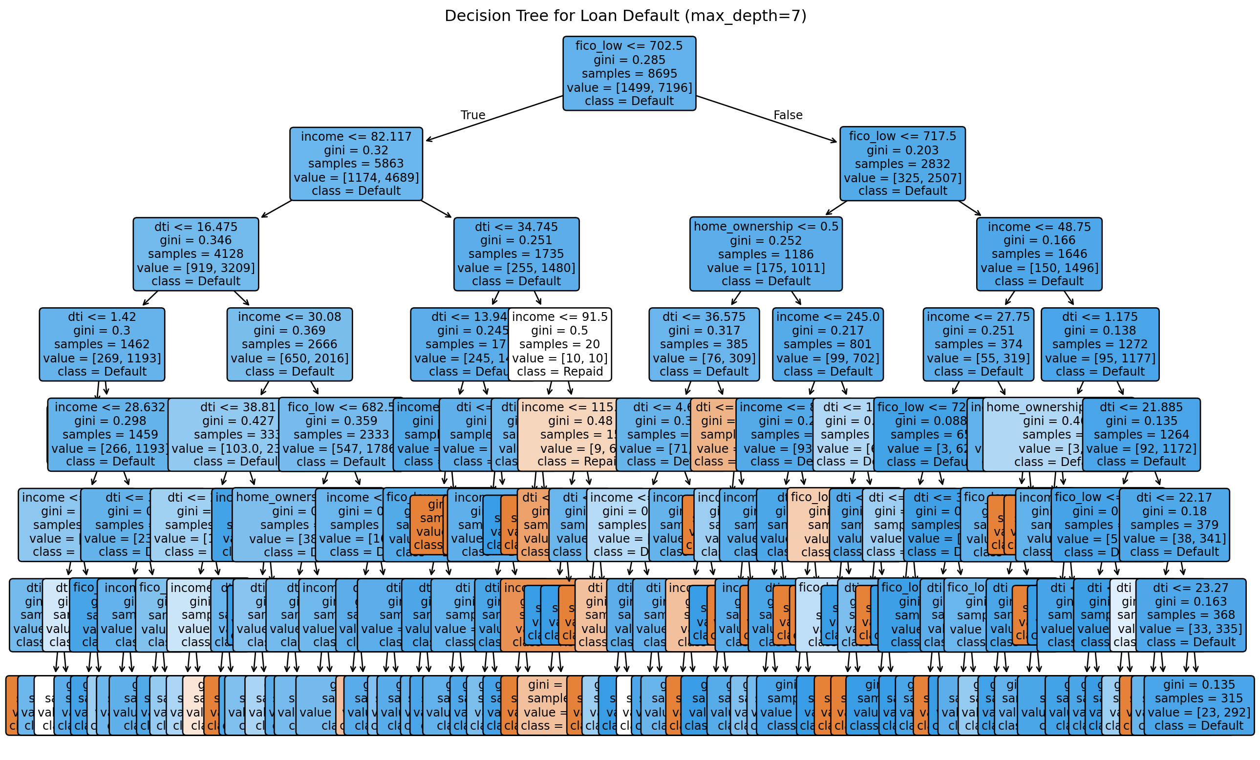
Visualizing the Learned Tree
The tree learns splits automatically from the data. Each node shows the split condition, impurity, sample count, and class distribution.
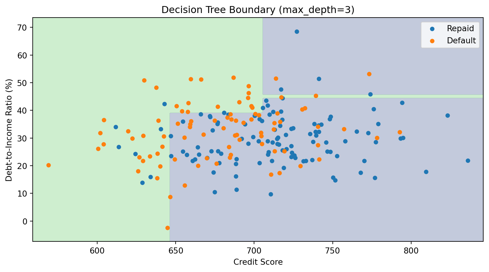
The Decision Boundary of a Tree
Decision tree boundaries are always axis-aligned rectangles—combinations of horizontal and vertical lines. This is a limitation compared to k-NN’s curved boundaries.
Controlling Tree Complexity
Deep trees can overfit—they memorize the training data perfectly but fail on new data.
Strategies to prevent overfitting:
Pre-pruning: Stop growing before the tree becomes too complex
max_depth: Maximum tree depth
min_samples_split: Minimum samples required to split a node
min_samples_leaf: Minimum samples required in a leaf
Post-pruning: Grow a full tree, then remove branches that don’t help
ccp_alpha: Cost-complexity pruning parameter
These hyperparameters are chosen via cross-validation.
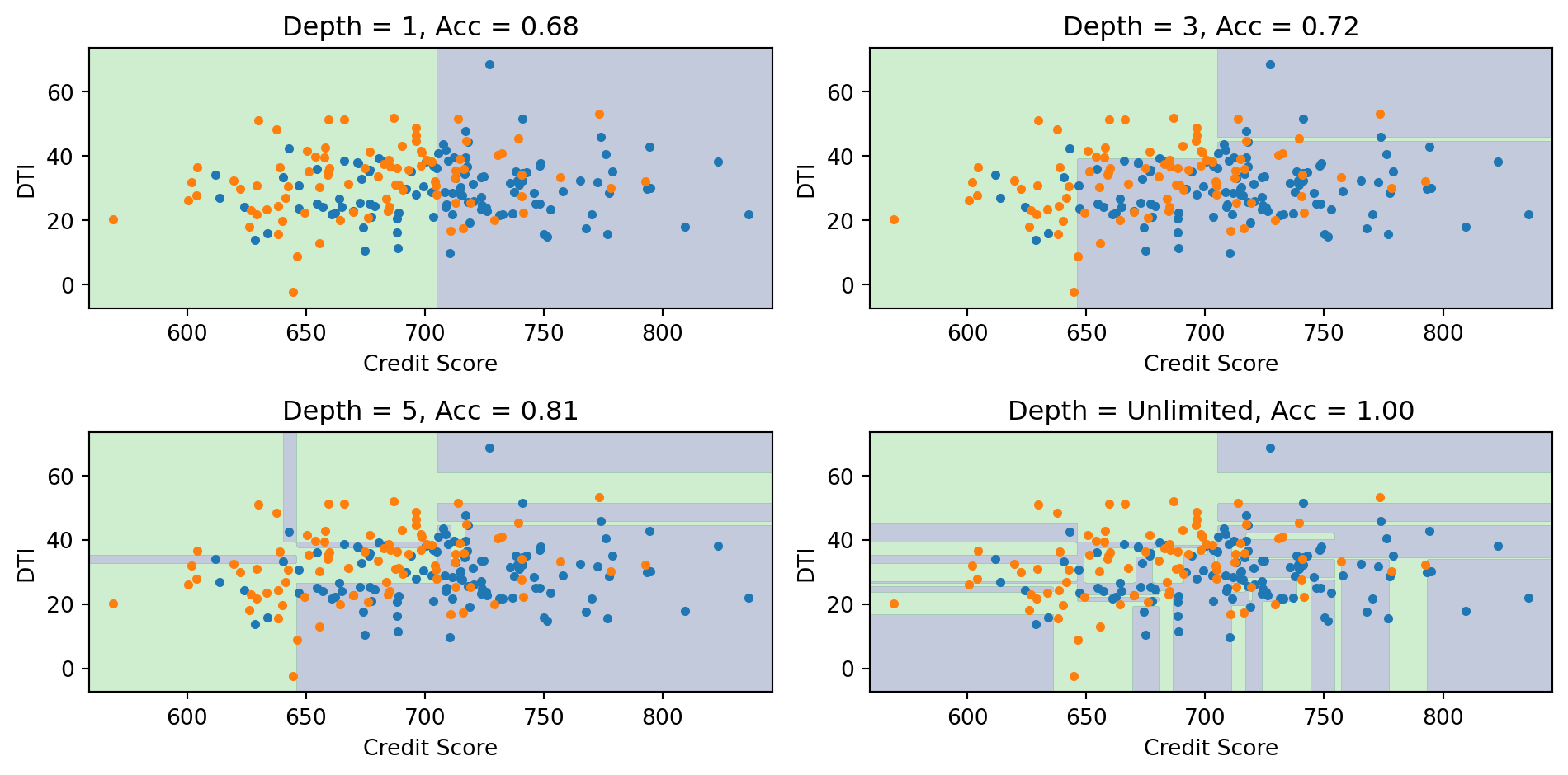
Effect of Tree Depth
Deeper trees create more complex boundaries. With unlimited depth, the tree can achieve 100% training accuracy but likely overfits.
Decision Trees: Advantages and Disadvantages
Advantages:
Easy to interpret and explain (white-box model)
Handles both numeric and categorical features
Requires little data preprocessing (no scaling needed)
Can capture interactions between features
Fast prediction
Disadvantages:
Axis-aligned boundaries only (can’t capture diagonal boundaries efficiently)
High variance—small changes in data can produce very different trees
Prone to overfitting without regularization
Greedy algorithm may not find globally optimal tree
The high variance problem is addressed by ensemble methods (Random Forests, Gradient Boosting)—we’ll cover these in Week 9.
Part III: Comparing k-NN and Decision Trees
k-NN vs. Decision Trees
Aspect
k-NN
Decision Trees
Decision boundary
Flexible, curved
Axis-aligned rectangles
Training
None (stores data)
Builds tree structure
Prediction speed
Slow (compare to all training)
Fast (traverse tree)
Interpretability
Low (black-box)
High (rules)
Feature scaling
Required
Not required
High dimensions
Struggles (curse of dim.)
Handles better
Missing data
Problematic
Can handle
Neither method dominates—the best choice depends on the data and application requirements.
When to Use k-NN
k-NN is a good choice when:
You have low to moderate dimensionality (say, \(p < 20\))
The decision boundary is expected to be complex and curved
Interpretability is not critical
You have enough computational resources for prediction
The data is relatively dense
Applications in finance:
Anomaly detection (fraudulent transactions look different from neighbors)
Collaborative filtering (recommend assets held by similar investors)
Pattern matching (find historical periods similar to current conditions)
When to Use Decision Trees
Decision trees are a good choice when:
Interpretability is important (need to explain decisions)
You have mixed feature types (numeric and categorical)
There may be complex interactions between features
Fast prediction is required
You’ll use them as building blocks for ensembles
Applications in finance:
Credit scoring (need explainable decisions for regulatory compliance)
Lending Club was a peer-to-peer lending platform where individuals could lend money to other individuals.
The classification problem: Given borrower characteristics at the time of application, predict whether the loan will be repaid or will default.
Features include:
FICO score (credit score, 300-850)
Annual income
Debt-to-income ratio (DTI)
Home ownership (own, mortgage, rent)
Loan amount
Employment length
This is a real business problem with significant financial stakes—approving a bad loan costs money, but rejecting a good loan loses revenue.
Loading and Preparing the Data
import pandas as pd# Load Lending Club data (pre-split by Hull)train_data = pd.read_excel('lendingclub_traindata.xlsx')test_data = pd.read_excel('lendingclub_testdata.xlsx')# Check columns and targetprint(f"Training samples: {len(train_data)}")print(f"Test samples: {len(test_data)}")print(f"\nTarget distribution in training data:")print(train_data['loan_status'].value_counts(normalize=True))
Training samples: 8695
Test samples: 5916

Target distribution in training data:
loan_status
1    0.827602
0    0.172398
Name: proportion, dtype: float64
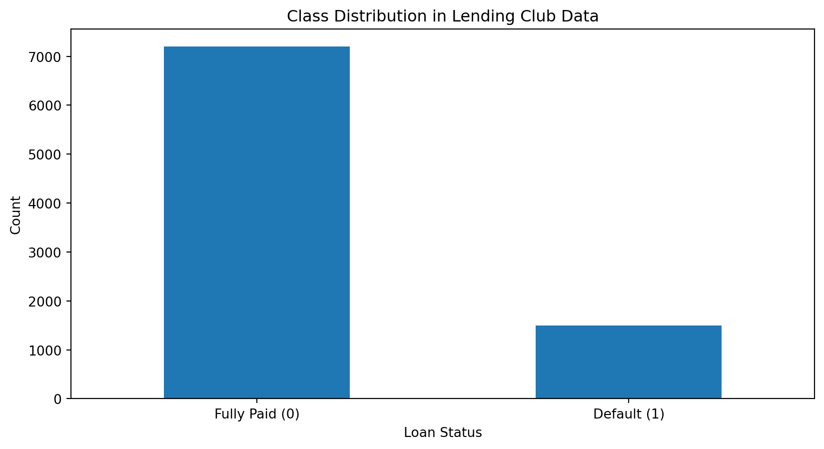
Class Imbalance
Fully paid: 17.2%
Default: 82.8%
The data is imbalanced: most loans are repaid. This is realistic—lenders wouldn’t survive if most loans defaulted!
Imbalanced data requires careful evaluation. High accuracy might just mean predicting “repaid” for everyone.
Preparing Features
# Select features for modelingfeatures = ['fico_low', 'income', 'dti', 'home_ownership']# Prepare X and yX_train = train_data[features].copy()y_train = train_data['loan_status'].valuesX_test = test_data[features].copy()y_test = test_data['loan_status'].values# Handle missing values if anyX_train = X_train.fillna(X_train.median())X_test = X_test.fillna(X_train.median())print(f"\nFeature summary:")print(X_train.describe())
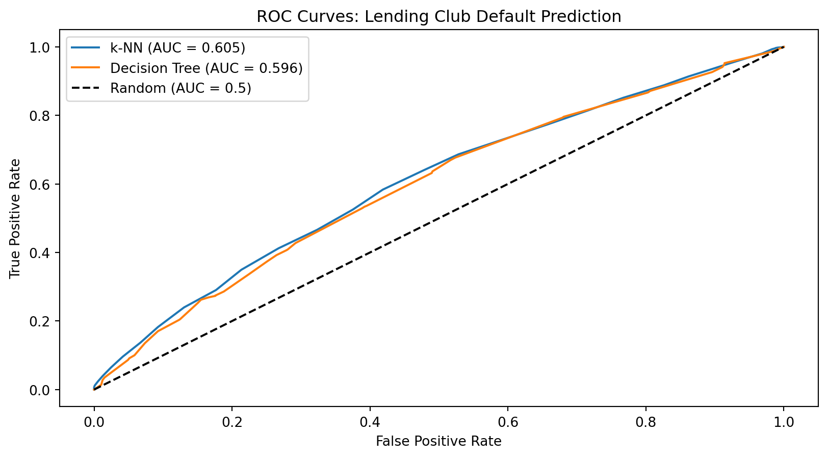
The ROC curve shows the tradeoff between catching defaults (true positive rate) and falsely flagging good loans (false positive rate).
Interpreting the Decision Tree
The tree reveals which features matter most. The first split (root) uses the most informative feature—likely FICO score, consistent with banking practice.
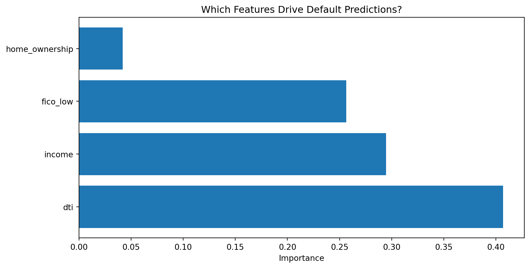
Feature Importance
import pandas as pd# Get feature importances from treeimportances = pd.DataFrame({'Feature': features,'Importance': tree_final.feature_importances_}).sort_values('Importance', ascending=False)print("Feature Importances (Decision Tree):")print(importances.to_string(index=False))