RSM338: Machine Learning in Finance

Week 7: Linear Classification | March 4–5, 2026

Kevin Mott

Rotman School of Management

Today’s Goal

This week we move from predicting continuous outcomes (regression) to predicting categorical outcomes (classification).

Classification in finance: credit default, fraud detection, market direction, bankruptcy prediction, sector assignment.

Today: logistic regression, linear discriminant analysis (LDA), and evaluation metrics.

The Binary Classification Setup

We have \(n\) observations, each with features \(\mathbf{x}_i\) and a binary class label \(y_i \in \{0, 1\}\).

Our goal: learn a function that predicts \(y\) for new observations.

Two approaches:

  1. Predict the class directly: Output 0 or 1
  2. Predict the probability: Estimate \(P(y = 1 \,|\, \mathbf{x})\), then threshold

The second approach is more flexible—it tells us how confident we are, not just the prediction.

Part I: Why Not Just Use Regression?

The Linear Probability Model

A natural first idea: encode \(y \in \{0, 1\}\) and fit linear regression. This is the linear probability model.

We’ll use credit card default data throughout this lecture: 1 million individuals with balance, income, and default status.

import numpy as np
import pandas as pd

# Load credit default data
data = pd.read_csv('credit_default.csv')

balance = data['balance'].values
income = data['income'].values
default = data['default'].values

print(f"Observations: {len(data)}")
print(f"Default rate: {default.mean():.1%}")
Observations: 1000000
Default rate: 3.3%
from sklearn.linear_model import LinearRegression

# Fit linear regression
X = balance.reshape(-1, 1)
y = default

lr = LinearRegression()
lr.fit(X, y)

# Predictions
balance_grid = np.linspace(0, 2700, 100).reshape(-1, 1)
prob_linear = lr.predict(balance_grid)

The Problem: Predictions Outside [0, 1]

The linear probability model can produce “probabilities” that aren’t valid probabilities.

prob_all = lr.predict(balance.reshape(-1, 1))

print(f"Minimum predicted probability: {prob_all.min():.3f}")
print(f"Maximum predicted probability: {prob_all.max():.3f}")
print(f"Number of predictions < 0: {(prob_all < 0).sum()}")
print(f"Number of predictions > 1: {(prob_all > 1).sum()}")
Minimum predicted probability: -0.106
Maximum predicted probability: 0.344
Number of predictions < 0: 330069
Number of predictions > 1: 0

What does a probability of -0.05 mean? These are nonsensical.

We need a function that naturally maps any input to the interval (0, 1). This is exactly what logistic regression does.

Part II: Logistic Regression

The Logistic Function

Instead of modeling probability as a linear function, we use the logistic function (also called the sigmoid function):

\[\sigma(z) = \frac{e^z}{1 + e^z} = \frac{1}{1 + e^{-z}}\]

This S-shaped function has two properties:

  1. Output is always between 0 and 1: \(\displaystyle\lim_{z \to -\infty} \sigma(z) = 0\); \(\displaystyle\lim_{z \to +\infty} \sigma(z) = 1\)
  2. Monotonic: Larger \(z\) always means larger probability

The Logistic Regression Model

In logistic regression, we model the probability of the positive class as:

\[P(y = 1 \,|\, \mathbf{x}) = \sigma(\beta_0 + \boldsymbol{\beta}' \mathbf{x}) = \frac{1}{1 + e^{-(\beta_0 + \boldsymbol{\beta}' \mathbf{x})}}\]

The notation \(P(y = 1 \,|\, \mathbf{x})\) reads “the probability that \(y = 1\) given \(\mathbf{x}\).” This is a conditional probability—the probability of default, given that we observe a particular set of feature values.

Here \(\mathbf{x} = (x_1, x_2, \ldots, x_p)'\) is a \(p\)-vector of features (attributes) for an observation, and \(\boldsymbol{\beta} = (\beta_1, \beta_2, \ldots, \beta_p)'\) is the corresponding \(p\)-vector of coefficients we need to learn.

The Linear Predictor

Let’s define \(z = \beta_0 + \boldsymbol{\beta}' \mathbf{x}\) as the linear predictor. Writing out the dot product:

\[z = \beta_0 + \beta_1 x_1 + \beta_2 x_2 + \cdots + \beta_p x_p\]

Then the model becomes:

\[P(y = 1 \,|\, \mathbf{x}) = \frac{1}{1 + e^{-z}}\]

The linear combination \(z\) can be any real number, but the logistic function squashes it to (0, 1).

  • If \(z = 0\): \(P(y=1) = 0.5\) (coin flip)
  • If \(z > 0\): \(P(y=1) > 0.5\) (more likely positive)
  • If \(z < 0\): \(P(y=1) < 0.5\) (more likely negative)

What Are Odds?

You’ve seen odds in sports betting: “the Leafs are 3-to-1 to win” means for every 1 time they win, they lose 3 times.

\[\text{Odds} = \frac{P(\text{event})}{P(\text{no event})} = \frac{P(\text{event})}{1 - P(\text{event})}\]

Probability Odds Interpretation
50% 1:1 Even money—equally likely
75% 3:1 3 times more likely to happen than not
20% 1:4 4 times more likely not to happen
90% 9:1 Very likely

Odds range from 0 to \(\infty\), with 1 being the “neutral” point (50-50). This asymmetry is awkward—log-odds fixes it.

The Log-Odds (Logit) Interpretation

Taking the log of odds gives us log-odds (also called the logit):

  • Log-odds of 0 means 50-50 (odds = 1)
  • Positive log-odds means more likely than not
  • Negative log-odds means less likely than not

In logistic regression, the log-odds is linear in the features:

\[\ln\left(\frac{P(y = 1 \,|\, \mathbf{x})}{1 - P(y = 1 \,|\, \mathbf{x})}\right) = \beta_0 + \boldsymbol{\beta}' \mathbf{x}\]

The coefficient \(\beta_j\) tells us how a one-unit increase in \(x_j\) affects the log-odds:

  • If \(\beta_j > 0\): higher \(x_j\) increases the probability of \(y = 1\)
  • If \(\beta_j < 0\): higher \(x_j\) decreases the probability of \(y = 1\)
  • If \(\beta_j = 0\): \(x_j\) has no effect

We can also interpret coefficients as odds ratios: \(e^{\beta_j}\) is the multiplicative change in odds for a one-unit increase in \(x_j\). If \(\beta_j = 0.5\), then \(e^{0.5} \approx 1.65\): each one-unit increase multiplies the odds by 1.65 (a 65% increase).

Fitting Logistic Regression: The Loss Function

How do we find the best coefficients \(\beta_0, \boldsymbol{\beta}\)? Like any ML model, we define a loss function and minimize it.

For observation \(i\) with features \(\mathbf{x}_i\) and label \(y_i\), let \(\hat{p}_i = P(y_i = 1 \,|\, \mathbf{x}_i)\) be our predicted probability. Intuitively:

  • If \(y_i = 1\): we want \(\hat{p}_i\) close to 1 (predict high probability for actual positives)
  • If \(y_i = 0\): we want \(\hat{p}_i\) close to 0 (predict low probability for actual negatives)

The binary cross-entropy loss (also called log loss) captures this:

\[\mathcal{L}(\boldsymbol{\beta}) = -\frac{1}{n}\sum_{i=1}^{n} \left[ y_i \ln(\hat{p}_i) + (1 - y_i) \ln(1 - \hat{p}_i) \right]\]

When \(y_i = 1\), the loss is \(-\ln(\hat{p}_i)\), which is small when \(\hat{p}_i\) is close to 1. When \(y_i = 0\), the loss is \(-\ln(1 - \hat{p}_i)\), which is small when \(\hat{p}_i\) is close to 0.

Comparing Loss Functions: Logistic vs. Linear Regression

Both linear and logistic regression fit into the same ML framework: define a loss function, then minimize it.

Linear Regression Logistic Regression
Output Continuous \(\hat{y}\) Probability \(\hat{p} \in (0,1)\)
Loss function Mean squared error (MSE) Binary cross-entropy
Formula \(\frac{1}{n}\sum_i (y_i - \hat{y}_i)^2\) \(-\frac{1}{n}\sum_i \left[ y_i \ln(\hat{p}_i) + (1-y_i)\ln(1-\hat{p}_i) \right]\)
Optimization Closed-form solution Iterative (gradient descent)

The choice of loss function depends on the problem: squared error makes sense for continuous outcomes, cross-entropy makes sense for probabilities.

Connection to statistics

In statistics, minimizing cross-entropy loss is equivalent to maximum likelihood estimation. Minimizing MSE is equivalent to maximum likelihood under the assumption that errors are normally distributed. Both approaches—ML and statistics—arrive at the same answer through different reasoning.

Logistic Regression for Credit Default

Let’s fit logistic regression to our credit default data:

from sklearn.linear_model import LogisticRegression

# Fit logistic regression
log_reg = LogisticRegression()
log_reg.fit(X, y)

# Predictions
prob_logistic = log_reg.predict_proba(balance_grid)[:, 1]

print(f"Logistic Regression:")
print(f"  Intercept: {log_reg.intercept_[0]:.4f}")
print(f"  Coefficient on balance: {log_reg.coef_[0, 0]:.6f}")
Logistic Regression:
  Intercept: -11.6163
  Coefficient on balance: 0.006383

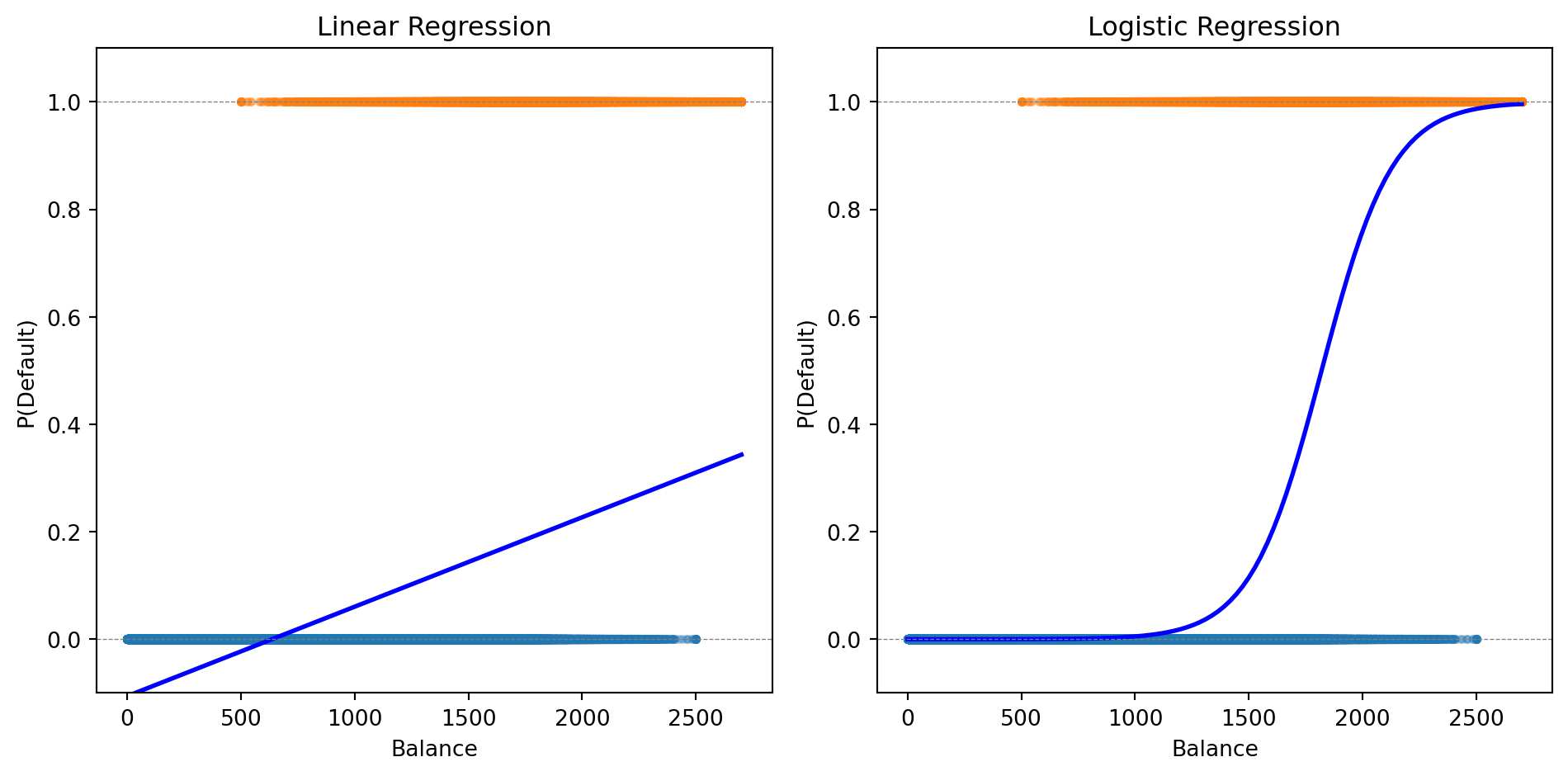
The logistic curve stays within [0, 1] and captures the S-shaped relationship between balance and default probability.

Making Predictions

Logistic regression gives us a probability. To make a classification decision, we need a threshold (also called a cutoff).

The default rule: predict class 1 if \(P(y = 1 \,|\, \mathbf{x}) > 0.5\)

# Predict probabilities and classes
prob_pred = log_reg.predict_proba(X)[:, 1]
class_pred = (prob_pred > 0.5).astype(int)

# Compare to actual
print(f"Using threshold = 0.5:")
print(f"  Predicted defaults: {class_pred.sum()}")
print(f"  Actual defaults: {int(default.sum())}")
print(f"  Correctly classified: {(class_pred == default).sum()} / {len(default)}")
print(f"  Accuracy: {(class_pred == default).mean():.1%}")
Using threshold = 0.5:
  Predicted defaults: 19005
  Actual defaults: 33000
  Correctly classified: 975591 / 1000000
  Accuracy: 97.6%

The 0.5 threshold isn’t always optimal—we’ll return to this when discussing evaluation metrics.

Multiple Features

Logistic regression easily extends to multiple predictors:

\[P(y = 1 \,|\, \mathbf{x}) = \frac{1}{1 + e^{-(\beta_0 + \beta_1 x_1 + \beta_2 x_2 + \cdots + \beta_p x_p)}}\]

# Fit with both balance and income
X_both = np.column_stack([balance, income])
log_reg_both = LogisticRegression()
log_reg_both.fit(X_both, default)

print(f"Logistic Regression with Balance and Income:")
print(f"  Intercept: {log_reg_both.intercept_[0]:.4f}")
print(f"  Coefficient on balance: {log_reg_both.coef_[0, 0]:.6f}")
print(f"  Coefficient on income: {log_reg_both.coef_[0, 1]:.9f}")
Logistic Regression with Balance and Income:
  Intercept: -11.2532
  Coefficient on balance: 0.006383
  Coefficient on income: -0.000009279

The coefficient on income is tiny—income adds little predictive power beyond balance.

Multi-Class Logistic Regression

When we have \(K > 2\) classes, we can extend logistic regression using the softmax function.

For each class \(k\), we define a linear predictor:

\[z_k = \beta_{k,0} + \boldsymbol{\beta}_k' \mathbf{x}\]

The probability of class \(k\) is:

\[P(y = k | \mathbf{x}) = \frac{e^{z_k}}{\sum_{j=1}^{K} e^{z_j}}\]

This is called multinomial logistic regression or softmax regression.

The softmax function ensures:

  • Each probability is between 0 and 1
  • The probabilities sum to 1 across all classes

Regularized Logistic Regression

Just like linear regression, logistic regression can overfit—especially with many features.

We can add regularization. Lasso logistic regression maximizes:

\[\mathcal{L}(\boldsymbol{\beta}) - \lambda \sum_{j=1}^{p} |\beta_j|\]

The penalty \(\lambda \sum |\beta_j|\) shrinks coefficients toward zero and can set some exactly to zero (variable selection).

Benefits:

  • Prevents overfitting when \(p\) is large relative to \(n\)
  • Identifies which features matter most
  • Improves out-of-sample prediction

The regularization parameter \(\lambda\) is chosen by cross-validation.

from sklearn.linear_model import LogisticRegressionCV

# Fit Lasso logistic regression with CV
log_reg_lasso = LogisticRegressionCV(penalty='l1', solver='saga', cv=5, max_iter=1000)
log_reg_lasso.fit(X_both, default)

print(f"Lasso Logistic Regression (λ chosen by CV):")
print(f"  Best C (inverse of λ): {log_reg_lasso.C_[0]:.4f}")
print(f"  Coefficient on balance: {log_reg_lasso.coef_[0, 0]:.6f}")
print(f"  Coefficient on income: {log_reg_lasso.coef_[0, 1]:.9f}")
Lasso Logistic Regression (λ chosen by CV):
  Best C (inverse of λ): 0.0001
  Coefficient on balance: 0.001064
  Coefficient on income: -0.000123506

Part III: Decision Boundaries

The Decision Boundary

Think of a classifier as drawing a line (or curve) through feature space that separates the classes. The decision boundary is this dividing line—observations on one side get predicted as Class 0, observations on the other side as Class 1.

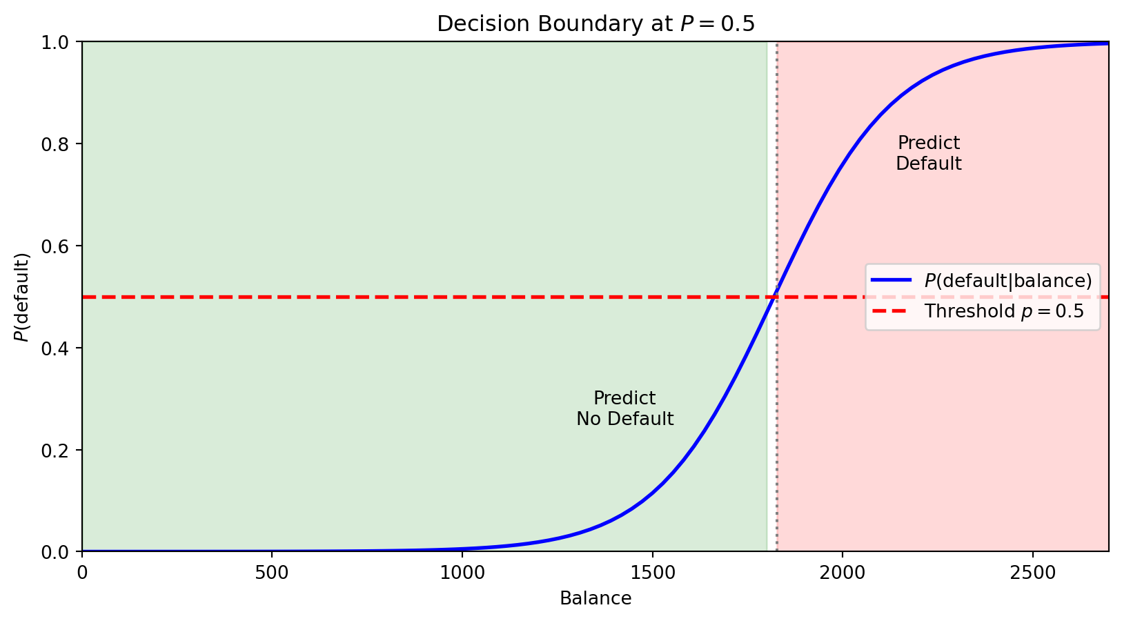
For logistic regression with threshold 0.5, we predict Class 1 when \(P(y = 1 \,|\, \mathbf{x}) > 0.5\).

The boundary is where \(P(y = 1 \,|\, \mathbf{x}) = 0.5\) exactly—the point of maximum uncertainty.

The horizontal red line marks \(P = 0.5\). Where the probability curve crosses this threshold defines the decision boundary in feature space—observations with balance above this point are predicted to default.

With multiple features, the boundary is where \(\beta_0 + \beta_1 x_1 + \beta_2 x_2 + \cdots = 0\)—a linear equation in the features. This is why logistic regression is called a linear classifier: the decision boundary is a line (in 2D) or hyperplane (in higher dimensions).

What If Classes Aren’t Linearly Separable?

Sometimes a straight line can’t separate the classes well. We can create curved boundaries by adding transformed features to our model:

  • Include \(x_1^2\), \(x_2^2\), \(x_1 x_2\) as additional features
  • The model is still logistic regression (linear in these new features)
  • But the boundary is now curved in the original \((x_1, x_2)\) space

We’ll see more flexible classifiers (trees, k-NN) next week that don’t require manual feature engineering.

The model is still “logistic regression” (linear in the transformed features), but the decision boundary is nonlinear in the original features.

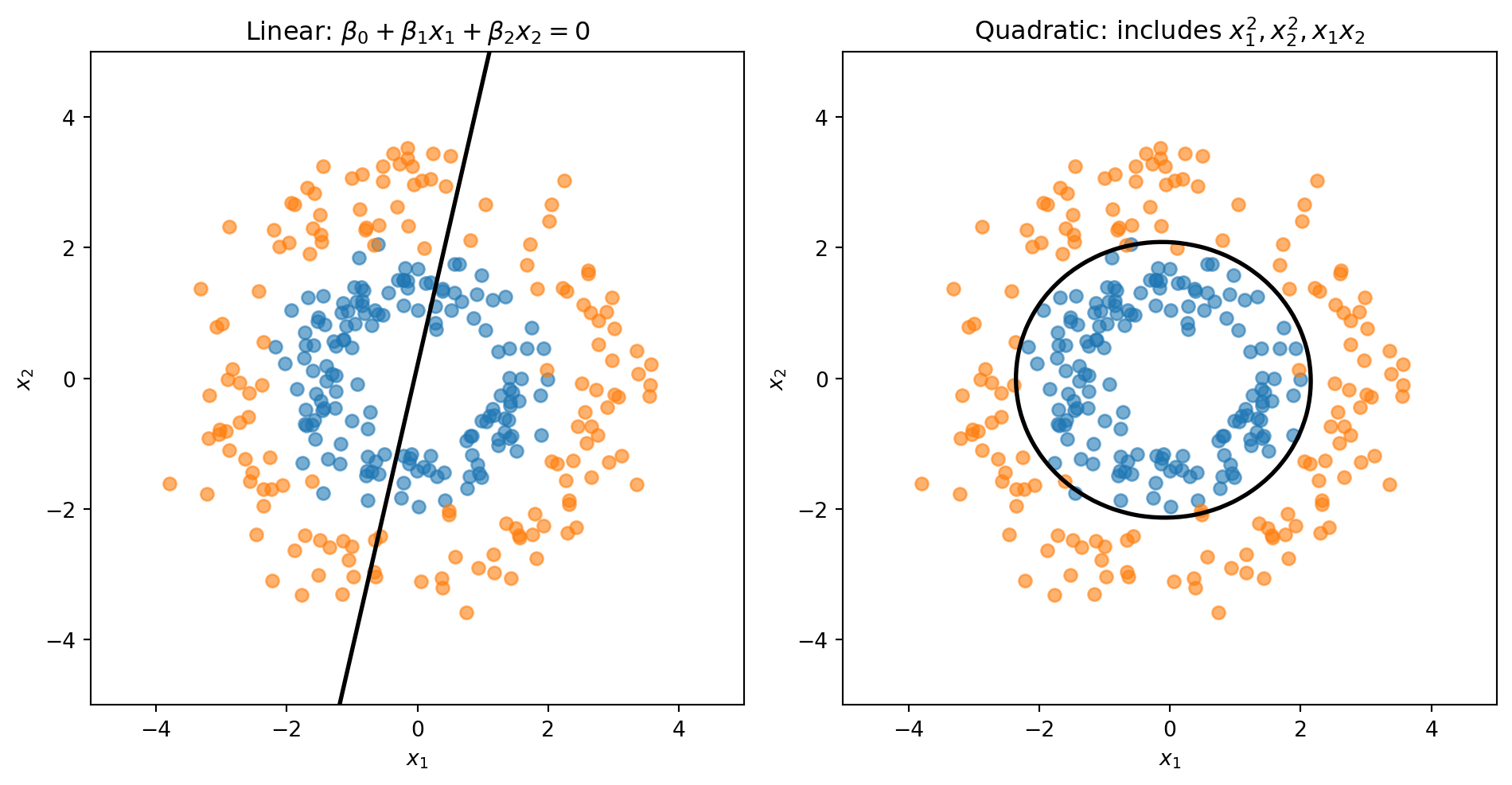
Linear vs. Quadratic Boundaries

Consider data where Class 0 forms an inner ring and Class 1 forms an outer ring. No straight line can separate these classes—we need a circular boundary.

A circle centered at the origin has equation \(x_1^2 + x_2^2 = r^2\). If we add squared terms as features, the decision boundary becomes:

\[\beta_0 + \beta_1 x_1 + \beta_2 x_2 + \beta_3 x_1^2 + \beta_4 x_1 x_2 + \beta_5 x_2^2 = 0\]

This is a quadratic equation in \(x_1\) and \(x_2\)—it can represent circles, ellipses, or other curved shapes.

from sklearn.preprocessing import PolynomialFeatures

# Linear: uses only x1, x2
log_reg_linear = LogisticRegression()
log_reg_linear.fit(X_ring, y_ring)

# Quadratic: add x1^2, x2^2, x1*x2 as new features
poly = PolynomialFeatures(degree=2)
X_ring_poly = poly.fit_transform(X_ring)
log_reg_quad = LogisticRegression()
log_reg_quad.fit(X_ring_poly, y_ring)
LogisticRegression()
In a Jupyter environment, please rerun this cell to show the HTML representation or trust the notebook.
On GitHub, the HTML representation is unable to render, please try loading this page with nbviewer.org.

To visualize the decision boundary, we create a grid of points, compute \(P(y=1)\) at each point, then draw the contour where \(P = 0.5\).

# Create grid covering the feature space
x1_range = np.linspace(-5, 5, 100)
x2_range = np.linspace(-5, 5, 100)
X1, X2 = np.meshgrid(x1_range, x2_range)
grid = np.column_stack([X1.ravel(), X2.ravel()])

# Predict P(y=1) at every grid point
probs_linear = log_reg_linear.predict_proba(grid)[:, 1].reshape(X1.shape)
probs_quad = log_reg_quad.predict_proba(poly.transform(grid))[:, 1].reshape(X1.shape)

The linear model is forced to draw a straight line through the rings. The quadratic model can learn a circular boundary that actually separates the classes.

Part IV: Linear Discriminant Analysis

Why Another Classifier?

Clustering (Week 5) Logistic Regression LDA
Type Unsupervised Supervised Supervised
Labels Unknown — discover them Known — learn a boundary Known — learn distributions
Strategy Assume each group is a distribution; find the groups Directly model \(P(y \mid \mathbf{x})\) Model \(P(\mathbf{x} \mid y)\) per class, then apply Bayes’ theorem

LDA is the supervised version of the distributional thinking you used in clustering: instead of discovering groups, you already know them and want to learn what makes each group different.

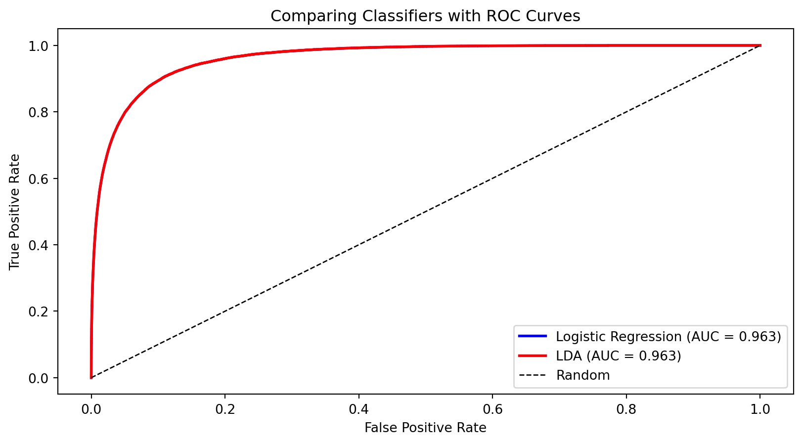
In practice, LDA and logistic regression often give similar answers — the value is in understanding both ways of thinking about classification.

A Different Approach: Bayes’ Theorem

Logistic regression directly models \(P(y | \mathbf{x})\)—the probability of the class given the features.

Discriminant analysis takes a different approach using Bayes’ theorem:

\[P(y = k | \mathbf{x}) = \frac{P(\mathbf{x} | y = k) \cdot P(y = k)}{P(\mathbf{x})}\]

In words:

\[\text{Posterior} = \frac{\text{Likelihood} \times \text{Prior}}{\text{Evidence}}\]

Instead of modeling \(P(y | \mathbf{x})\) directly, we model:

  • \(P(y = k)\) — the prior probability of each class (how common is each class?)
  • \(P(\mathbf{x} | y = k)\) — the likelihood (what do features look like within each class?)

Setting Up the Model

Let’s establish notation:

  • \(K\) classes labeled \(1, 2, \ldots, K\)
  • \(\pi_k = P(y = k)\) — prior probability of class \(k\)
  • \(f_k(\mathbf{x}) = P(\mathbf{x} | y = k)\) — probability density of \(\mathbf{x}\) given class \(k\)

Bayes’ theorem gives us the posterior probability:

\[P(y = k | \mathbf{x}) = \frac{f_k(\mathbf{x}) \pi_k}{\sum_{j=1}^{K} f_j(\mathbf{x}) \pi_j}\]

The denominator is the same for all classes—it just ensures probabilities sum to 1.

We classify to the class with the highest posterior probability.

The Normality Assumption

Linear Discriminant Analysis (LDA) assumes that within each class, the features follow a multivariate normal distribution:

\[\mathbf{X} \,|\, y = k \;\sim\; \mathcal{N}(\boldsymbol{\mu}_k, \boldsymbol{\Sigma})\]

The density function is:

\[f_k(\mathbf{x}) = \frac{1}{(2\pi)^{p/2} |\boldsymbol{\Sigma}|^{1/2}} \exp\left(-\frac{1}{2}(\mathbf{x} - \boldsymbol{\mu}_k)' \boldsymbol{\Sigma}^{-1}(\mathbf{x} - \boldsymbol{\mu}_k)\right)\]

where:

  • \(\boldsymbol{\mu}_k\) is the mean of class \(k\) (different for each class)
  • \(\boldsymbol{\Sigma}\) is the covariance matrix (same for all classes — this is the key assumption!)

Each class is a normal “blob” centered at \(\boldsymbol{\mu}_k\), but all classes share the same shape (covariance).

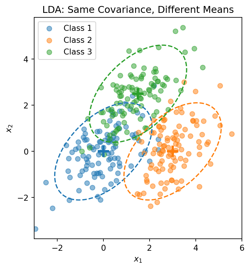
Visualizing the LDA Assumption

The dashed ellipses show the 95% probability contours—they have the same shape (orientation and spread) but different centers.

The LDA Discriminant Function

Start with the posterior from Bayes’ theorem:

\[P(y = k \,|\, \mathbf{x}) = \frac{f_k(\mathbf{x}) \pi_k}{\sum_{j=1}^{K} f_j(\mathbf{x}) \pi_j}\]

Taking the log and plugging in the normal density:

\[\ln P(y = k \,|\, \mathbf{x}) = \ln f_k(\mathbf{x}) + \ln \pi_k - \underbrace{\ln \sum_{j} f_j(\mathbf{x}) \pi_j}_{\text{same for all } k}\]

The normal density gives \(\ln f_k(\mathbf{x}) = -\frac{p}{2}\ln(2\pi) - \frac{1}{2}\ln|\boldsymbol{\Sigma}| - \frac{1}{2}(\mathbf{x} - \boldsymbol{\mu}_k)'\boldsymbol{\Sigma}^{-1}(\mathbf{x} - \boldsymbol{\mu}_k)\).

The first two terms don’t depend on \(k\) (shared covariance!). Expanding the quadratic and dropping terms that don’t depend on \(k\), we get the discriminant function:

\[\delta_k(\mathbf{x}) = \mathbf{x}' \boldsymbol{\Sigma}^{-1} \boldsymbol{\mu}_k - \frac{1}{2}\boldsymbol{\mu}_k' \boldsymbol{\Sigma}^{-1} \boldsymbol{\mu}_k + \ln \pi_k\]

This is a scalar—one number for each class \(k\). We classify \(\mathbf{x}\) to the class with the largest discriminant: \(\hat{y} = \arg\max_k \delta_k(\mathbf{x})\).

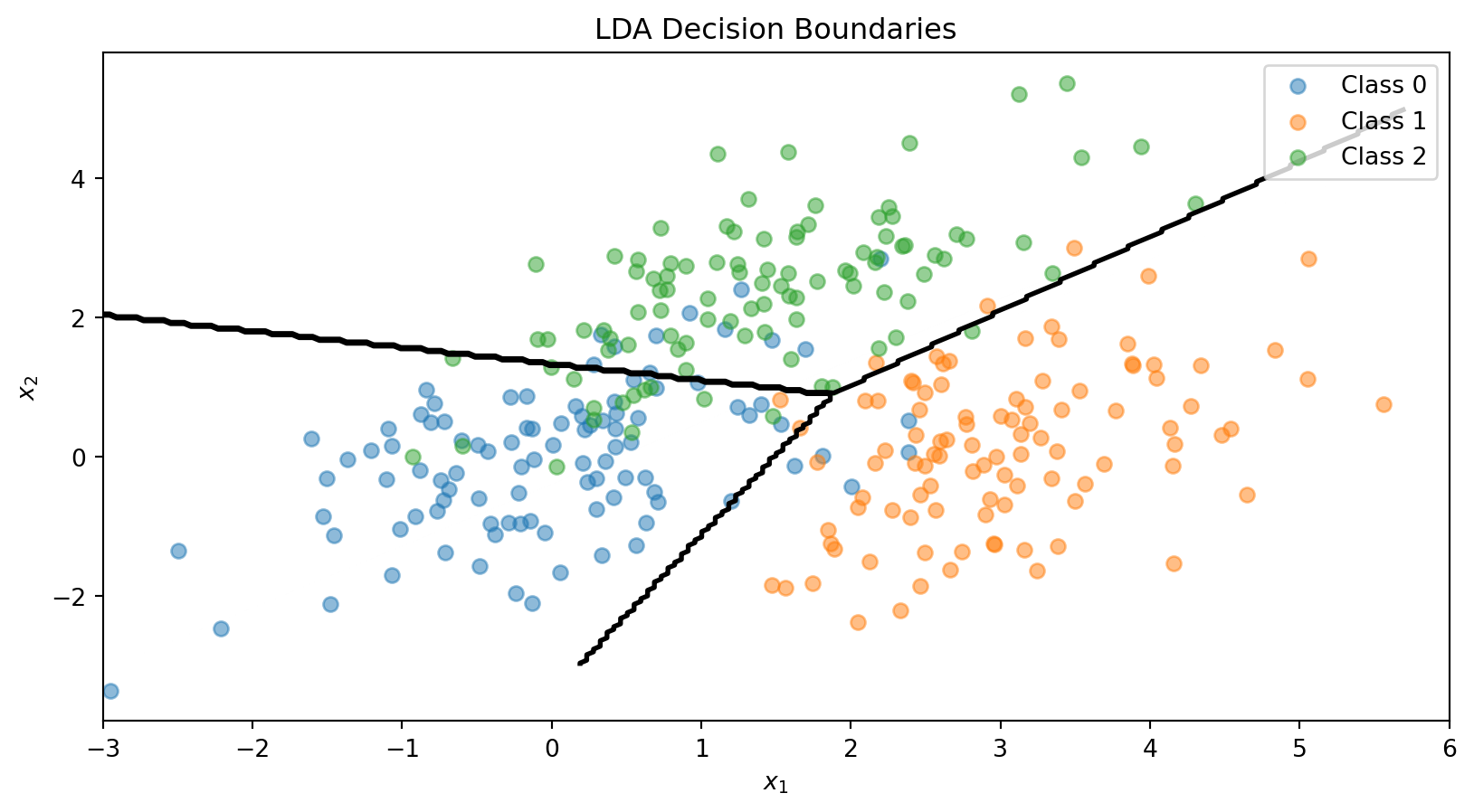
The discriminant function is linear in \(\mathbf{x}\)—that’s why it’s called Linear Discriminant Analysis.

The LDA Decision Boundary

The decision boundary between classes \(k\) and \(\ell\) is where:

\[\delta_k(\mathbf{x}) = \delta_\ell(\mathbf{x})\]

This simplifies to:

\[\mathbf{x}' \boldsymbol{\Sigma}^{-1} (\boldsymbol{\mu}_k - \boldsymbol{\mu}_\ell) = \frac{1}{2}(\boldsymbol{\mu}_k' \boldsymbol{\Sigma}^{-1} \boldsymbol{\mu}_k - \boldsymbol{\mu}_\ell' \boldsymbol{\Sigma}^{-1} \boldsymbol{\mu}_\ell) + \ln\frac{\pi_\ell}{\pi_k}\]

This is a linear equation in \(\mathbf{x}\)—so the boundary is a line (in 2D) or hyperplane (in higher dimensions).

With \(K\) classes, we have \(K(K-1)/2\) pairwise boundaries, but only \(K-1\) of them matter for defining the decision regions.

Estimating LDA Parameters

In practice, we estimate the parameters from training data:

Prior probabilities: \[\hat{\pi}_k = \frac{n_k}{n}\]

where \(n_k\) is the number of training observations in class \(k\).

Class means: \[\hat{\boldsymbol{\mu}}_k = \frac{1}{n_k} \sum_{i: y_i = k} \mathbf{x}_i\]

Pooled covariance matrix: \[\hat{\boldsymbol{\Sigma}} = \frac{1}{n - K} \sum_{k=1}^{K} \sum_{i: y_i = k} (\mathbf{x}_i - \hat{\boldsymbol{\mu}}_k)(\mathbf{x}_i - \hat{\boldsymbol{\mu}}_k)'\]

The pooled covariance averages within-class covariances, weighted by class size.

The LDA Recipe

LDA
Model Each class \(k\) is a multivariate normal: \(\mathbf{x} \mid y = k \;\sim\; \mathcal{N}(\boldsymbol{\mu}_k,\, \boldsymbol{\Sigma})\)
Parameters Priors \(\hat{\pi}_k = n_k / n\), means \(\hat{\boldsymbol{\mu}}_k\), pooled covariance \(\hat{\boldsymbol{\Sigma}}\)
“Loss function” Not a loss function — parameters are estimated directly from the data (sample proportions, sample means, pooled covariance)
Classification rule Assign \(\mathbf{x}\) to the class with the largest discriminant \(\delta_k(\mathbf{x})\)

No optimization loop, no gradient descent. LDA computes its parameters in closed form — plug in the training data and you’re done.

This is fundamentally different from logistic regression, which iteratively searches for the coefficients that minimize cross-entropy loss.

LDA in Python

from sklearn.discriminant_analysis import LinearDiscriminantAnalysis

# Combine the 3-class data
X_lda = np.vstack([X1, X2, X3])
y_lda = np.array([0] * n_per_class + [1] * n_per_class + [2] * n_per_class)

# Fit LDA
lda = LinearDiscriminantAnalysis()
lda.fit(X_lda, y_lda)

print("LDA Class Means:")
for k in range(3):
    print(f"  Class {k}: {lda.means_[k]}")

print(f"\nClass Priors: {lda.priors_}")
LDA Class Means:
  Class 0: [ 0.00962094 -0.02608294]
  Class 1: [3.00835928 0.12294623]
  Class 2: [1.40152169 2.3715806 ]

Class Priors: [0.33333333 0.33333333 0.33333333]
# Visualize LDA decision boundaries
fig, ax = plt.subplots()

ax.scatter(X1[:, 0], X1[:, 1], alpha=0.5, label='Class 0')
ax.scatter(X2[:, 0], X2[:, 1], alpha=0.5, label='Class 1')
ax.scatter(X3[:, 0], X3[:, 1], alpha=0.5, label='Class 2')

# Decision boundaries
x_range = np.linspace(-3, 6, 200)
y_range = np.linspace(-3, 5, 200)
X_grid, Y_grid = np.meshgrid(x_range, y_range)
grid_points = np.column_stack([X_grid.ravel(), Y_grid.ravel()])
Z = lda.predict(grid_points).reshape(X_grid.shape)

ax.contour(X_grid, Y_grid, Z, levels=[0.5, 1.5], colors='black', linewidths=2)
ax.set_xlabel('$x_1$')
ax.set_ylabel('$x_2$')
ax.set_title('LDA Decision Boundaries')
ax.legend()
plt.show()

Quadratic Discriminant Analysis (QDA)

LDA assumes all classes share the same covariance matrix \(\boldsymbol{\Sigma}\).

Quadratic Discriminant Analysis (QDA) relaxes this: each class has its own covariance \(\boldsymbol{\Sigma}_k\).

The discriminant function becomes:

\[\delta_k(\mathbf{x}) = -\frac{1}{2}\ln|\boldsymbol{\Sigma}_k| - \frac{1}{2}(\mathbf{x} - \boldsymbol{\mu}_k)' \boldsymbol{\Sigma}_k^{-1}(\mathbf{x} - \boldsymbol{\mu}_k) + \ln \pi_k\]

This is quadratic in \(\mathbf{x}\), giving curved decision boundaries.

Trade-off:

  • LDA: More restrictive assumptions, fewer parameters to estimate, more stable
  • QDA: More flexible, more parameters, can overfit with small samples

LDA vs. QDA

When classes have different covariances, QDA captures the curved boundary while LDA is forced to use a straight line.

Why LDA Works Well

LDA and QDA have good track records as classifiers, not necessarily because the normality assumption is correct, but because:

  1. Stability: Estimating fewer parameters (shared \(\boldsymbol{\Sigma}\)) reduces variance
  2. Robustness: The decision boundary often works well even when normality is violated
  3. Closed-form solution: No iterative optimization needed

When to use which:

  • LDA: When you have limited data or classes are well-separated
  • QDA: When you have more data and suspect different class shapes
  • Regularized DA: Blend between LDA and QDA to control flexibility

LDA vs. Logistic Regression

Both produce linear decision boundaries. When to use which?

Logistic Regression:

  • Makes no assumption about the distribution of \(\mathbf{x}\)
  • More robust when the normality assumption is violated
  • Preferred when you have binary features or mixed feature types

LDA:

  • More efficient when normality holds (uses information about class distributions)
  • Can be more stable with small samples
  • Naturally handles multi-class problems

In practice, they often give similar results. Try both and compare via cross-validation.

Part V: Evaluating Classification Models

Beyond Accuracy

For regression, we use MSE or \(R^2\) to measure performance.

For classification, accuracy (% correct) is the obvious metric:

\[\text{Accuracy} = \frac{\text{Number Correct}}{\text{Total}} = \frac{TP + TN}{TP + TN + FP + FN}\]

But accuracy can be misleading, especially with imbalanced classes.

Example: Predicting credit card fraud (1% fraud rate)

  • A model that predicts “not fraud” for everyone achieves 99% accuracy!
  • But it catches zero fraud cases—useless for the actual goal.

We need metrics that account for different types of errors.

The Confusion Matrix

A confusion matrix summarizes all prediction outcomes:

Actual Positive Actual Negative
Predicted Positive True Positive (TP) False Positive (FP)
Predicted Negative False Negative (FN) True Negative (TN)
  • True Positive (TP): Correctly predicted positive
  • False Positive (FP): Incorrectly predicted positive (Type I error)
  • True Negative (TN): Correctly predicted negative
  • False Negative (FN): Incorrectly predicted positive as negative (Type II error)

Different applications care about different cells of this matrix.

Key Metrics from the Confusion Matrix

Accuracy: Overall correct rate \[\text{Accuracy} = \frac{TP + TN}{TP + TN + FP + FN}\]

Precision: Of those we predicted positive, how many actually are? \[\text{Precision} = \frac{TP}{TP + FP}\]

Recall (Sensitivity): Of the actual positives, how many did we catch? \[\text{Recall} = \frac{TP}{TP + FN}\]

Specificity: Of the actual negatives, how many did we correctly identify? \[\text{Specificity} = \frac{TN}{TN + FP}\]

False Positive Rate: Of actual negatives, how many did we wrongly call positive? \[\text{FPR} = \frac{FP}{TN + FP} = 1 - \text{Specificity}\]

Credit Default: Confusion Matrix

from sklearn.metrics import confusion_matrix, classification_report

# Using our credit default data with logistic regression
y_pred = log_reg.predict(X)

# Confusion matrix
cm = confusion_matrix(default, y_pred)
print("Confusion Matrix:")
print(f"                  Predicted No  Predicted Yes")
print(f"  Actual No          {cm[0,0]:5d}         {cm[0,1]:5d}")
print(f"  Actual Yes         {cm[1,0]:5d}         {cm[1,1]:5d}")
Confusion Matrix:
                  Predicted No  Predicted Yes
  Actual No          961793          5207
  Actual Yes         19202         13798
# Metrics
TP = cm[1, 1]
TN = cm[0, 0]
FP = cm[0, 1]
FN = cm[1, 0]

print(f"\nMetrics:")
print(f"  Accuracy:    {(TP + TN) / (TP + TN + FP + FN):.1%}")
print(f"  Precision:   {TP / (TP + FP):.1%}" if (TP + FP) > 0 else "  Precision: N/A")
print(f"  Recall:      {TP / (TP + FN):.1%}")
print(f"  Specificity: {TN / (TN + FP):.1%}")

Metrics:
  Accuracy:    97.6%
  Precision:   72.6%
  Recall:      41.8%
  Specificity: 99.5%

The Class Imbalance Problem

With 97% non-defaulters and 3% defaulters, the model is biased toward predicting “no default.”

Using threshold = 0.5, we have high accuracy (97%+) but low recall—we miss most actual defaults.

For a credit card company, missing defaults is costly! They’d rather:

  • Catch more actual defaults (higher recall)
  • Even if it means more false alarms (lower precision)

The 0.5 threshold isn’t sacred—we can adjust it based on business needs.

Adjusting the Classification Threshold

Instead of predicting “default” when \(P(\text{default}) > 0.5\), we can use a lower threshold:

Predict “default” when \(P(\text{default}) > \tau\)

Lower threshold \(\tau\):

  • More predictions of “default”
  • Higher recall (catch more true defaults)
  • Lower precision (more false alarms)

Higher threshold \(\tau\):

  • Fewer predictions of “default”
  • Lower recall (miss more true defaults)
  • Higher precision (fewer false alarms)

Effect of Threshold Choice

# Try different thresholds
thresholds = [0.5, 0.2, 0.1, 0.05]
prob_pred = log_reg.predict_proba(X)[:, 1]

print("Effect of Threshold on Confusion Matrix Metrics:\n")
print(f"{'Threshold':>10} {'Accuracy':>10} {'Precision':>10} {'Recall':>10} {'FPR':>10}")
print("-" * 52)

for thresh in thresholds:
    y_pred_thresh = (prob_pred > thresh).astype(int)
    cm = confusion_matrix(default, y_pred_thresh)
    TP, TN, FP, FN = cm[1,1], cm[0,0], cm[0,1], cm[1,0]

    acc = (TP + TN) / (TP + TN + FP + FN)
    prec = TP / (TP + FP) if (TP + FP) > 0 else 0
    rec = TP / (TP + FN)
    fpr = FP / (TN + FP)

    print(f"{thresh:>10.2f} {acc:>10.1%} {prec:>10.1%} {rec:>10.1%} {fpr:>10.1%}")
Effect of Threshold on Confusion Matrix Metrics:

 Threshold   Accuracy  Precision     Recall        FPR
----------------------------------------------------
      0.50      97.6%      72.6%      41.8%       0.5%
      0.20      96.7%      50.2%      66.0%       2.2%
      0.10      94.9%      37.0%      78.1%       4.5%
      0.05      91.7%      26.7%      86.7%       8.1%

Lowering the threshold from 0.5 to 0.1 dramatically increases recall (catching defaults) at the cost of more false positives.
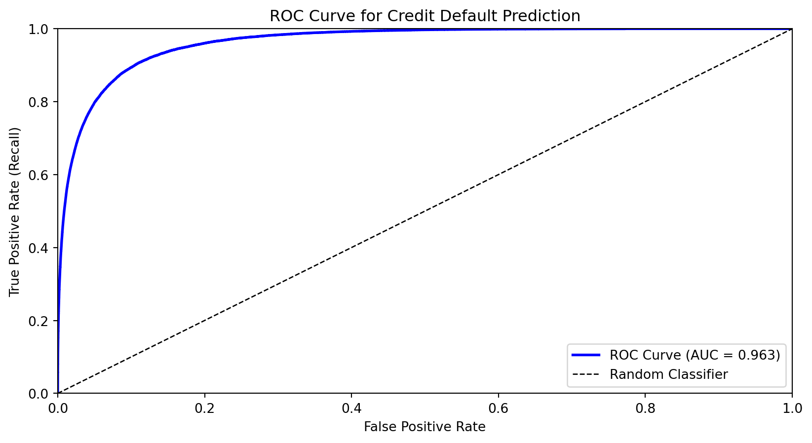
The ROC Curve

The Receiver Operating Characteristic (ROC) curve shows the trade-off between true positive rate (recall) and false positive rate across all thresholds.

  • X-axis: False Positive Rate (FPR)
  • Y-axis: True Positive Rate (TPR = Recall)

As we lower the threshold:

  • We move from bottom-left (predict nothing positive) toward top-right (predict everything positive)
  • Good classifiers hug the top-left corner

Area Under the ROC Curve (AUC)

The Area Under the Curve (AUC) summarizes the ROC curve in a single number:

  • AUC = 1.0: Perfect classifier
  • AUC = 0.5: Random guessing (diagonal line)
  • AUC < 0.5: Worse than random (predictions inverted)

Interpretation: AUC is the probability that a randomly chosen positive example is ranked higher than a randomly chosen negative example.

from sklearn.metrics import roc_auc_score

auc = roc_auc_score(default, prob_pred)
print(f"AUC for credit default model: {auc:.3f}")
AUC for credit default model: 0.963

AUC is useful for comparing models because it’s threshold-independent—it measures the model’s ability to rank observations correctly.

Choosing the Optimal Threshold

The “best” threshold depends on the costs of different errors:

  • Cost of false negative (missing a default): \(c_{FN}\)
  • Cost of false positive (false alarm): \(c_{FP}\)

If missing defaults is very costly (e.g., the bank loses the loan amount), we want a lower threshold to maximize recall.

Objective: Minimize total cost \[\text{Total Cost} = c_{FN} \cdot FN + c_{FP} \cdot FP\]

Or equivalently, maximize: \[\text{Benefit} = TP - c \cdot FP\]

where \(c = c_{FP} / c_{FN}\) is the relative cost ratio.

Comparing Classifiers

The ROC curves are nearly identical—both methods perform similarly on this dataset. The AUC provides a single number for comparison.

Summary and Preview

What We Learned Today

Classification predicts categorical outcomes—a core supervised learning task.

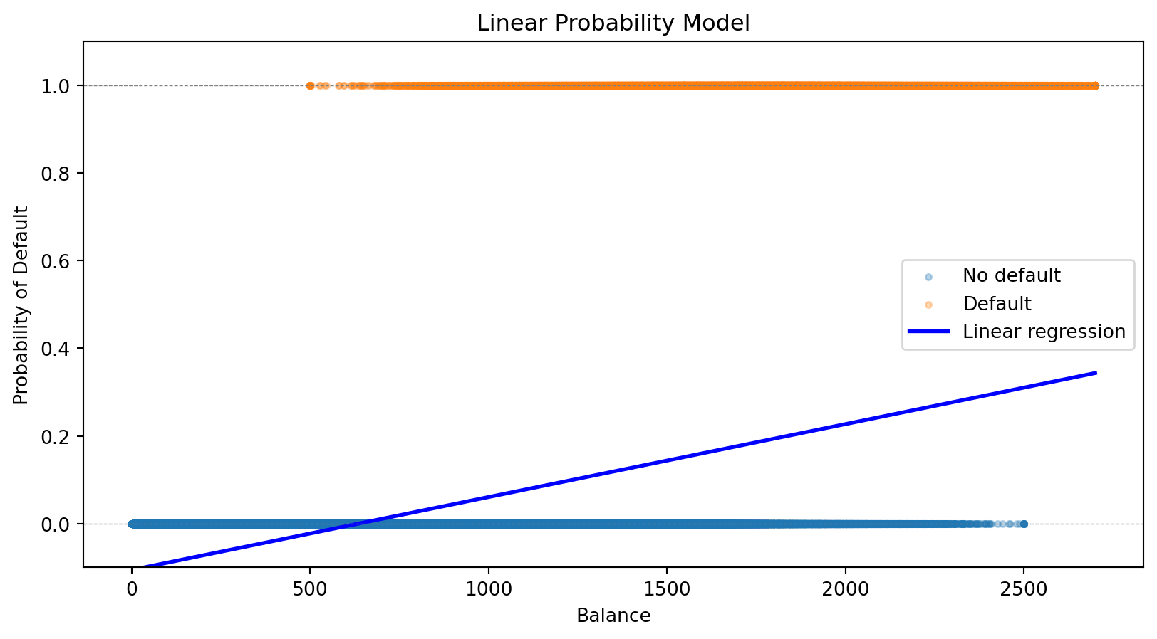
Linear probability model (regression with 0/1 outcome) fails because it can produce impossible probabilities.

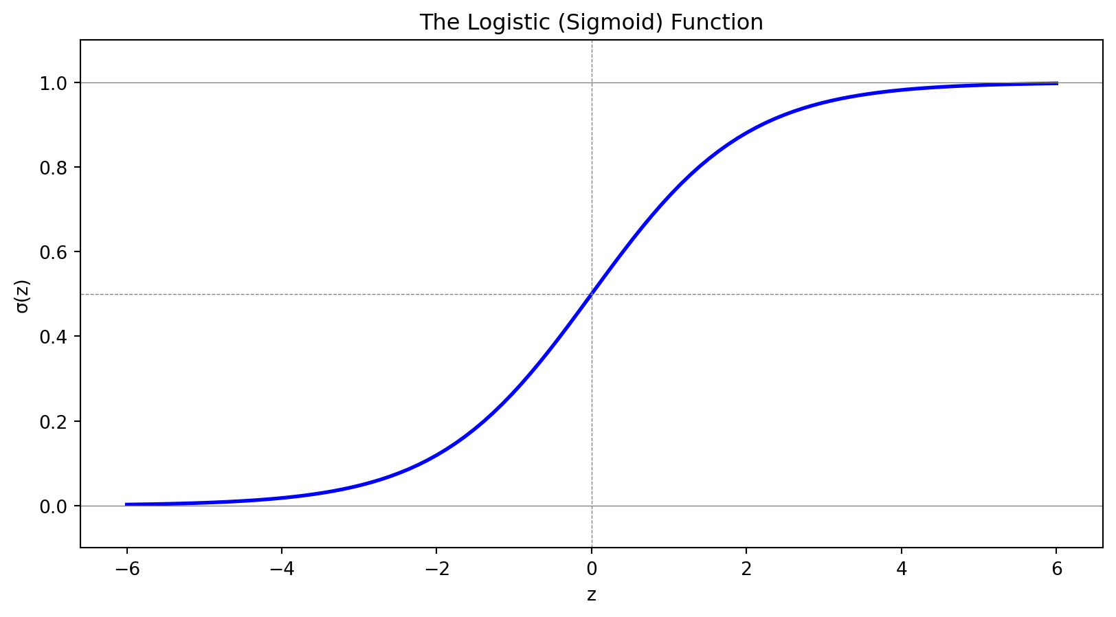
Logistic regression uses the sigmoid function to model probabilities properly:

  • Outputs are always in (0, 1)
  • Coefficients measure effect on log-odds
  • Can be regularized (Lasso) for variable selection

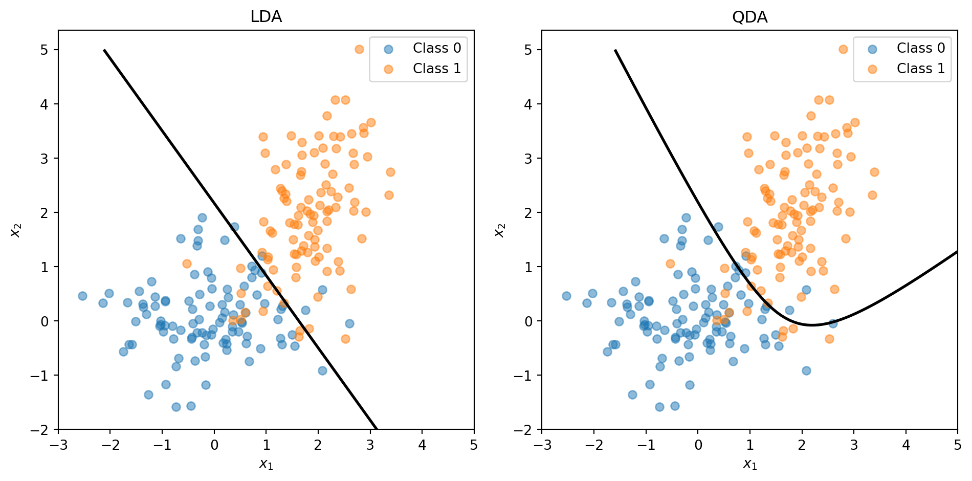
Linear Discriminant Analysis takes a Bayesian approach:

  • Models class-conditional distributions as normal
  • Assumes shared covariance (LDA) or class-specific covariance (QDA)
  • Often performs similarly to logistic regression

Evaluation Metrics

Accuracy can be misleading with imbalanced classes.

The confusion matrix breaks down predictions into TP, FP, TN, FN.

Precision (of predicted positives, how many are correct?) and Recall (of actual positives, how many did we catch?) capture different aspects of performance.

The ROC curve shows the trade-off across all thresholds.

AUC summarizes discriminative ability in a single number.

The optimal threshold depends on the costs of different types of errors.

Next Week

Week 8: Nonlinear Classification

We’ll extend to methods that create nonlinear decision boundaries:

  • k-Nearest Neighbors (k-NN): Classify based on nearby training points
  • Decision Trees: Recursive partitioning of feature space
  • Support Vector Machines: Find the maximum margin boundary

These methods can capture complex patterns that linear classifiers miss.

References

  • Fisher, R. A. (1936). The use of multiple measurements in taxonomic problems. Annals of Eugenics, 7(2), 179-188.
  • Hastie, T., Tibshirani, R., & Friedman, J. (2009). The Elements of Statistical Learning (2nd ed.). Springer. Chapter 4.
  • James, G., Witten, D., Hastie, T., & Tibshirani, R. (2021). An Introduction to Statistical Learning (2nd ed.). Springer. Chapter 4.