RSM338: Machine Learning in Finance

Week 6: ML and Portfolio Theory | February 11–12, 2026

Kevin Mott

Rotman School of Management

Today’s Goal

Last week we learned about regression and regularization. This week we connect machine learning to a core finance problem: portfolio optimization.

The problem: We want to invest optimally, but we don’t know the true expected returns and covariances—we have to estimate them from data.

Today’s roadmap:

1. Mean-variance utility: How do investors evaluate portfolios?
2. Optimal portfolios: Finding the best weights for single and multiple assets
3. The estimation problem: True parameters vs. estimated parameters
4. Estimation risk: Why optimized portfolios often disappoint
5. ML solutions: Using regularization (Lasso) to improve portfolio performance

Recall: Mean-Variance Utility

From RSM332: investors care about the expected return and risk (variance) of their portfolio. Mean-variance utility captures this trade-off:

\[U = \underbrace{\mathbb{E}[R_p]}_{\text{expected return}} - \frac{\gamma}{2} \underbrace{\text{Var}(R_p)}_{\text{risk}}\]

where \(\gamma > 0\) is the risk aversion parameter — how much the investor dislikes variance. Higher \(\gamma\) means more risk-averse: you demand more expected return to compensate for a given level of risk.

The investor wants to maximize this utility: earn as high a return as possible, penalized by how much risk they take on.

Empirical estimates suggest typical investors have \(\gamma\) between 2 and 10. For \(\gamma = 2\): accepting 1% more variance requires roughly 1% more expected return to maintain the same utility.

The utility value has a concrete interpretation: the certainty equivalent — the guaranteed (risk-free) return that would make the investor indifferent between holding the risky portfolio or receiving that guaranteed return for sure. A risk-averse investor’s certainty equivalent is always below the expected return.

Recall: Portfolio Mean and Variance

Suppose you hold \(N\) risky assets with weights \(w_1, w_2, \ldots, w_N\). Let \(r_i\) denote the excess return of asset \(i\) (return above the risk-free rate). The portfolio excess return is \(r_p = w_1 r_1 + w_2 r_2 + \cdots + w_N r_N\).

Expected excess return is the weighted average of individual expected excess returns:

\[\mathbb{E}[r_p] = \sum_{i=1}^{N} w_i \, \mathbb{E}[r_i]\]

Variance includes both individual variances and all pairwise covariances:

\[\text{Var}(r_p) = \sum_{i=1}^{N} \sum_{j=1}^{N} w_i \, w_j \, \text{Cov}(r_i, r_j)\]

In vector notation, stacking everything into vectors and matrices:

\[\mathbb{E}[r_p] = \mathbf{w}^\top \boldsymbol{\mu} \qquad \text{Var}(r_p) = \mathbf{w}^\top \boldsymbol{\Sigma} \mathbf{w}\]

where \(\mathbf{w}\) is the \(N \times 1\) weight vector on risky assets only, \(\boldsymbol{\mu}\) is the \(N \times 1\) vector of expected excess returns, and \(\boldsymbol{\Sigma}\) is the \(N \times N\) covariance matrix. We don’t require \(\mathbf{w}^\top \mathbf{1} = 1\) — the remainder \(1 - \mathbf{w}^\top \mathbf{1}\) is invested in the risk-free asset. So mean-variance utility becomes:

\[U = \mathbf{w}^\top \boldsymbol{\mu} - \frac{\gamma}{2} \mathbf{w}^\top \boldsymbol{\Sigma} \mathbf{w}\]

Maximizing this gives the MVO solution:

\[\mathbf{w}^* = \frac{1}{\gamma} \boldsymbol{\Sigma}^{-1} \boldsymbol{\mu}\]

Advanced: Deriving the MVO Solution

To find the maximum, take the gradient with respect to \(\mathbf{w}\) and set it to zero. Using matrix calculus rules \(\frac{\partial}{\partial \mathbf{w}}(\mathbf{w}^\top \mathbf{a}) = \mathbf{a}\) and \(\frac{\partial}{\partial \mathbf{w}}(\mathbf{w}^\top \mathbf{A} \mathbf{w}) = 2\mathbf{A}\mathbf{w}\) (for symmetric \(\mathbf{A}\)):

\[\nabla_{\mathbf{w}} U = \boldsymbol{\mu} - \gamma \boldsymbol{\Sigma} \mathbf{w} = \mathbf{0}\]

Solving for \(\mathbf{w}\): \(\gamma \boldsymbol{\Sigma} \mathbf{w} = \boldsymbol{\mu} \implies \mathbf{w}^* = \frac{1}{\gamma} \boldsymbol{\Sigma}^{-1} \boldsymbol{\mu}\)

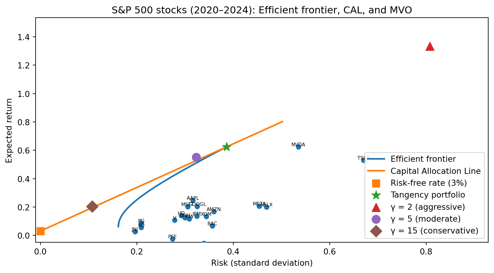
Recall: From Efficient Frontier to Optimal Portfolio

In RSM332, you built up to mean-variance optimization in three steps:

1. Efficient frontier — Given \(N\) risky assets, trace out the set of portfolios that offer the highest expected return for each level of risk. These are the “best available” combinations of risky assets.

2. Capital Allocation Line (CAL) — Introduce a risk-free asset. Now the investor can mix the risk-free asset with the tangency portfolio (the point where the CAL is tangent to the efficient frontier). The CAL gives the best possible risk-return trade-off.

3. Optimal portfolio choice — Where on the CAL does the investor land? That depends on preferences — their risk aversion \(\gamma\). A more risk-averse investor (\(\gamma\) high) holds more of the risk-free asset and less of the tangency portfolio. A less risk-averse investor (\(\gamma\) low) holds more risky assets, possibly leveraging.

Notice the MVO solution: \(\boldsymbol{\Sigma}^{-1} \boldsymbol{\mu}\) gives the tangency portfolio weights — the same for every investor. The scalar \(\frac{1}{\gamma}\) just scales how much you invest in it versus the risk-free asset. Every optimal investor holds the same risky portfolio, just in different amounts. That’s why they all land on the same line (the CAL).

Recall: The Power of Diversification

The correlation between assets determines how much diversification helps. Lower correlation means more risk reduction.

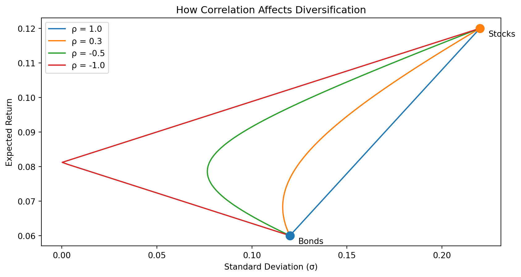
With \(\rho = 1\) (perfect correlation), there’s no diversification benefit — the opportunity set is a straight line. As correlation decreases, the curve bends left, offering the same return with less risk.

Why Revisit Mean-Variance Optimization?

The MVO solution \(\mathbf{w}^* = \frac{1}{\gamma} \boldsymbol{\Sigma}^{-1} \boldsymbol{\mu}\) is elegant — but it has a hidden assumption: you need to know \(\boldsymbol{\mu}\) and \(\boldsymbol{\Sigma}\).

In practice, you must estimate them from data. Recall from Week 2: plugging in estimates \(\hat{\mu}\) and \(\hat{\sigma}^2\) in place of the true parameters introduces estimation risk — additional uncertainty because our parameters are estimates, not truth. In Week 2, we saw this bias wealth forecasts upward. Here the consequences are worse: the MVO formula amplifies estimation error. Small errors in \(\hat{\boldsymbol{\mu}}\) and \(\hat{\boldsymbol{\Sigma}}\) get multiplied through the matrix inverse \(\boldsymbol{\Sigma}^{-1}\), producing wildly unstable portfolio weights.

This is the same “nearly singular inverse blows up” problem from Week 5 — but now it’s your money on the line.

The Gap Between Theory and Practice

In RSM332 (theory):

• \(\boldsymbol{\mu}\) and \(\boldsymbol{\Sigma}\) are known constants
• The optimization formula gives the truly optimal portfolio
• More assets = better diversification = higher utility

In practice:

• \(\boldsymbol{\mu}\) and \(\boldsymbol{\Sigma}\) must be estimated from noisy historical data
• The “optimal” portfolio is optimal for the estimated parameters, not the true ones
• More assets = more parameters to estimate = more estimation error = worse performance

This is one of the biggest puzzles in applied finance: theoretically optimal portfolios often perform worse than naive strategies like equal weighting.

Today we’ll understand why, and how machine learning helps.

Part I: Single Risky Asset

Portfolio with One Risky Asset

Consider the simplest case: you can invest in one risky asset (say, a stock index) and a risk-free asset (T-bills).

Let \(w\) be the fraction of your wealth invested in the risky asset. Then \((1 - w)\) is invested in the risk-free asset.

Let \(r_t\) denote the excess return of the risky asset at time \(t\). The excess return is the return above the risk-free rate:

\[r_t = R_t - R_f\]

where \(R_t\) is the total return and \(R_f\) is the risk-free rate.

Working with excess returns simplifies notation because the risk-free part of the portfolio contributes nothing to excess return.

Portfolio Mean and Variance

The excess return of the portfolio is simply:

\[r_{p,t} = w \cdot r_t\]

If you invest 60% in the risky asset (\(w = 0.6\)), your portfolio’s excess return is 60% of the risky asset’s excess return.

Taking expectations and using the properties from Week 1:

Expected excess return: \[\mu_p = w \cdot \mu\]

Variance: \[\sigma_p^2 = w^2 \cdot \sigma^2\]

Standard deviation: \[\sigma_p = |w| \cdot \sigma\]

Here \(\mu\) and \(\sigma^2\) are the expected excess return and variance of the risky asset.

The Sharpe Ratio

Notice something interesting. When \(w > 0\) (positive investment in the risky asset):

\[\frac{\mu_p}{\sigma_p} = \frac{w \cdot \mu}{w \cdot \sigma} = \frac{\mu}{\sigma}\]

The ratio of expected return to standard deviation is constant, regardless of how much you invest!

This ratio \(\frac{\mu}{\sigma}\) is the Sharpe ratio of the risky asset. From RSM332, you may recall that the Sharpe ratio measures the “reward per unit of risk.”

By adjusting \(w\), you can move along a straight line in risk-return space, but you can’t improve the Sharpe ratio—it’s determined by the risky asset itself.

Finding the Optimal Weight

The investor’s problem: choose \(w\) to maximize utility.

Substituting the portfolio mean and variance into the utility function:

\[U(w) = w\mu - \frac{\gamma}{2} w^2 \sigma^2\]

This is a quadratic function of \(w\)—it opens downward (because the coefficient on \(w^2\) is negative), so it has a unique maximum.

To find the maximum, we take the derivative with respect to \(w\) and set it equal to zero:

\[\frac{dU}{dw} = \mu - \gamma w \sigma^2 = 0\]

Solving for \(w\):

\[w^* = \frac{1}{\gamma} \cdot \frac{\mu}{\sigma^2}\]

Interpreting the Optimal Weight

The optimal weight formula:

\[w^* = \frac{1}{\gamma} \cdot \frac{\mu}{\sigma^2}\]

Let’s interpret each piece:

• \(\frac{1}{\gamma}\): Less risk-averse investors (\(\gamma\) smaller) invest more in the risky asset
• \(\mu\): Higher expected return \(\rightarrow\) invest more
• \(\frac{1}{\sigma^2}\): Higher variance \(\rightarrow\) invest less

The ratio \(\frac{\mu}{\sigma^2}\) is sometimes called the “reward-to-variance” ratio.

This is the foundation of mean-variance analysis, developed by Harry Markowitz in the 1950s—work that earned him the Nobel Prize in Economics.

Working with Real Data

Let’s compute the optimal weight using actual S&P 500 data:

import pandas as pd
import numpy as np

# Load S&P 500 data and compute annual total returns
sp500 = pd.read_csv('sp500_yf.csv', parse_dates=['Date'], index_col='Date')
annual_prices = sp500['Close'].resample('YE').last()
annual_returns = annual_prices.pct_change().dropna()

# Load risk-free rate (10-year Treasury yield, in percent)
rf_data = pd.read_csv('DGS10.csv', parse_dates=['observation_date'], index_col='observation_date')
rf_data['DGS10'] = pd.to_numeric(rf_data['DGS10'], errors='coerce')
rf_annual = rf_data['DGS10'].resample('YE').mean() / 100

# Excess returns = total return minus risk-free rate
excess_returns = (annual_returns - rf_annual).dropna()

# Estimate mean and variance of excess returns
mu_hat = excess_returns.mean()
sigma_hat = excess_returns.std()
sigma2_hat = sigma_hat ** 2

print(f"Sample period: {excess_returns.index[0].year} - {excess_returns.index[-1].year}")
print(f"Number of years: T = {len(excess_returns)}")
print(f"Mean excess return:  μ̂ = {mu_hat:.2%}")
print(f"Standard deviation:  σ̂ = {sigma_hat:.2%}")
print(f"Variance:           σ̂² = {sigma2_hat:.4f}")

Sample period: 1962 - 2025
Number of years: T = 64
Mean excess return:  μ̂ = 2.88%
Standard deviation:  σ̂ = 16.58%
Variance:           σ̂² = 0.0275

Computing the Optimal Weight

Now apply the formula \(w^* = \frac{1}{\gamma} \cdot \frac{\mu}{\sigma^2}\):

# Optimal weight depends on risk aversion
gamma = 2  # moderate risk aversion
w_star = (1 / gamma) * (mu_hat / sigma2_hat)

print(f"With γ = {gamma}:")
print(f"  w* = (1/{gamma}) × ({mu_hat:.4f} / {sigma2_hat:.4f})")
print(f"  w* = {w_star:.2f}")
print(f"\nInterpretation: invest {w_star:.0%} in stocks, {1-w_star:.0%} in T-bills")

With γ = 2:
  w* = (1/2) × (0.0288 / 0.0275)
  w* = 0.52

Interpretation: invest 52% in stocks, 48% in T-bills

# More risk-averse investor
gamma = 4
w_star_g4 = (1 / gamma) * (mu_hat / sigma2_hat)

print(f"With γ = {gamma}:")
print(f"  w* = {w_star_g4:.2f}")
print(f"\nInterpretation: invest {w_star_g4:.0%} in stocks, {1-w_star_g4:.0%} in T-bills")

With γ = 4:
  w* = 0.26

Interpretation: invest 26% in stocks, 74% in T-bills

Visualizing the Optimal Portfolio

import matplotlib.pyplot as plt

# Compare different risk aversion levels
gammas = [2, 4, 10]
w_range = np.linspace(-0.5, 3.0, 100)

plt.figure()
for gamma in gammas:
    # Compute utility curve for this gamma
    utility = w_range * mu_hat - (gamma / 2) * w_range**2 * sigma2_hat

    # Compute optimal weight
    w_star = (1 / gamma) * (mu_hat / sigma2_hat)
    u_star = w_star * mu_hat - (gamma / 2) * w_star**2 * sigma2_hat

    # Plot utility curve and optimal point
    plt.plot(w_range, utility, label=f'γ = {gamma}, w* = {w_star:.2f}')
    plt.scatter([w_star], [u_star], s=100, zorder=5)

plt.axhline(y=0, linestyle='-', lw=0.5)
plt.xlabel('Weight on risky asset (w)')
plt.ylabel('Utility U(w)')
plt.title('Higher risk aversion → lower optimal stock weight')
plt.legend()
plt.show()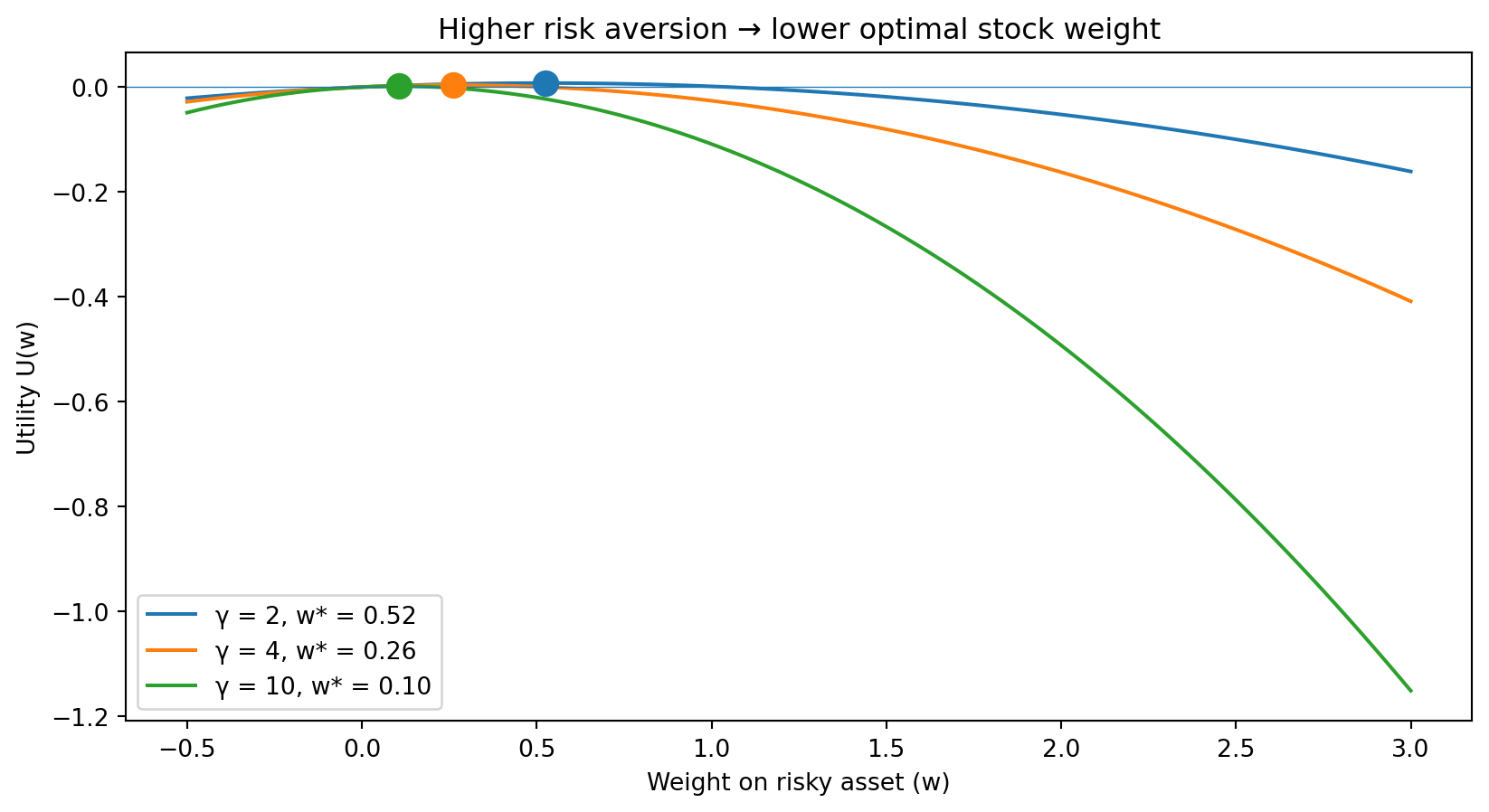

Higher risk aversion (larger \(\gamma\)) means more penalty for variance, so the investor holds less of the risky asset. The utility curves become more “curved” (more concave) as \(\gamma\) increases.

The Achieved Utility

What utility does the investor achieve at the optimal weight?

Substituting \(w^* = \frac{\mu}{\gamma \sigma^2}\) back into the utility function:

\[\begin{align*} U(w^*) &= w^* \mu - \frac{\gamma}{2} (w^*)^2 \sigma^2 \\ &= \frac{\mu}{\gamma \sigma^2} \cdot \mu - \frac{\gamma}{2} \cdot \frac{\mu^2}{\gamma^2 \sigma^4} \cdot \sigma^2 \\ &= \frac{\mu^2}{\gamma \sigma^2} - \frac{\mu^2}{2\gamma \sigma^2} \\ &= \frac{\mu^2}{2\gamma \sigma^2} \end{align*}\]

We can write this more compactly using the Sharpe ratio \(\theta = \frac{\mu}{\sigma}\):

\[U(w^*) = \frac{\theta^2}{2\gamma}\]

Part II: The Estimation Problem

From Theory to Practice

The optimal weight formula is elegant:

\[w^* = \frac{\mu}{\gamma \sigma^2}\]

But there’s a problem: we don’t know \(\mu\) and \(\sigma^2\).

These are the “true” population parameters—the expected return and variance that would emerge from the underlying probability distribution of returns.

In practice, we have historical data and must estimate these parameters. The estimates are denoted with “hats”:

• \(\hat{\mu}\) — the estimated expected return
• \(\hat{\sigma}^2\) — the estimated variance

Estimating Expected Return

Given \(T\) historical excess returns \(r_1, r_2, \ldots, r_T\), the natural estimate of expected return is the sample mean:

\[\hat{\mu} = \frac{1}{T} \sum_{t=1}^{T} r_t\]

In words: average the historical returns.

This is an unbiased estimator—on average, it equals the true \(\mu\). But any particular estimate \(\hat{\mu}\) will differ from \(\mu\) due to randomness in the sample.

The estimate varies from sample to sample. This variability is the source of estimation risk.

How Precise Is Our Estimate?

How confident should we be in our \(\hat{\mu}\)? Let’s construct a 95% confidence interval:

from scipy import stats
import numpy as np

# We already have annual_returns from earlier
T = len(annual_returns)

# Standard error of the mean
se = sigma_hat / np.sqrt(T)

# 95% confidence interval using t-distribution
t_crit = stats.t.ppf(0.975, T - 1)
ci_low = mu_hat - t_crit * se
ci_high = mu_hat + t_crit * se

print(f"Sample size: T = {T} years")
print(f"Standard error: SE = σ̂/√T = {sigma_hat:.4f}/√{T} = {se:.4f}")
print(f"Critical value: t₀.₉₇₅,{T-1} = {t_crit:.3f}")
print(f"\n95% Confidence Interval for μ:")
print(f"  ({ci_low:.2%}, {ci_high:.2%})")
print(f"\nEven with {T} years of data, we can't pin down μ!")

Sample size: T = 75 years
Standard error: SE = σ̂/√T = 0.1658/√75 = 0.0191
Critical value: t₀.₉₇₅,74 = 1.993

95% Confidence Interval for μ:
  (-0.93%, 6.70%)

Even with 75 years of data, we can't pin down μ!

The Uncertainty Is Huge

import matplotlib.pyplot as plt

fig, ax = plt.subplots()

# Plot the confidence interval
ax.errorbar([0], [mu_hat], yerr=[[mu_hat - ci_low], [ci_high - mu_hat]],
            fmt='o', capsize=10, capthick=2, markersize=10)
ax.axhline(y=mu_hat, linestyle='--', label=f'Point estimate: {mu_hat:.1%}')
ax.set_xlim(-0.5, 0.5)
ax.set_ylim(0, 0.20)
ax.set_ylabel('Expected Excess Return')
ax.set_xticks([])
ax.set_title(f'95% CI for expected excess return: [{ci_low:.1%}, {ci_high:.1%}]')
ax.legend()
plt.show()

print(f"Width of CI: {ci_high - ci_low:.1%}")
print("This is an enormous range for investment decisions!")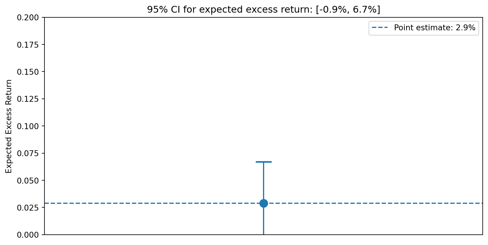

Width of CI: 7.6%
This is an enormous range for investment decisions!

Why Is Expected Return So Hard to Estimate?

The precision of our estimate depends on:

1. Sample size (\(T\)): More data helps, but improvement is slow (\(\frac{1}{\sqrt{T}}\))
2. Volatility (\(\sigma\)): Higher volatility means more noise, making estimation harder

# Signal-to-noise ratio for stocks is terrible
print(f"Mean excess return (signal):  {mu_hat:.1%}")
print(f"Std deviation (noise):    {sigma_hat:.1%}")
print(f"Signal-to-noise ratio:    {mu_hat/sigma_hat:.2f}")

Mean excess return (signal):  2.9%
Std deviation (noise):    16.6%
Signal-to-noise ratio:    0.17

The expected return is small relative to the volatility. To cut our uncertainty in half, we’d need four times as much data!

This is why Goyal and Welch (2008) found that most return predictors fail out-of-sample—expected returns are simply very hard to estimate.

Estimation Uncertainty Propagates to Weights

If we use the estimated mean to compute the optimal weight:

\[\hat{w} = \frac{\hat{\mu}}{\gamma \sigma^2}\]

(For now, assume \(\sigma^2\) is known.)

Under the assumption that returns are i.i.d. normal:

\[\hat{\mu} \sim N\left(\mu, \frac{\sigma^2}{T}\right)\]

Since \(\hat{w}\) is proportional to \(\hat{\mu}\), it inherits this uncertainty:

\[\hat{w} \sim N\left(w^*, \frac{1}{T \gamma^2 \sigma^2}\right)\]

The estimated weight varies around the true optimal weight \(w^*\).

How Wrong Can the Weight Be?

The uncertainty in \(\mu\) translates directly into uncertainty about the optimal weight:

gamma = 4

# Optimal weight at each end of the confidence interval
w_low = ci_low / (gamma * sigma2_hat)
w_high = ci_high / (gamma * sigma2_hat)

print(f"95% CI for μ: ({ci_low:.2%}, {ci_high:.2%})")
print(f"\nWith γ = {gamma}, the optimal weight w* = μ / (γσ²) could be:")
print(f"  If μ = {ci_low:.2%}:  w* = {ci_low:.4f} / ({gamma} × {sigma2_hat:.4f}) = {w_low:.2f}")
print(f"  If μ = {ci_high:.2%}: w* = {ci_high:.4f} / ({gamma} × {sigma2_hat:.4f}) = {w_high:.2f}")
print(f"\nRange of plausible weights: ({w_low:.0%}, {w_high:.0%})")
print(f"\nThis is a huge range for such a basic investment decision!")

95% CI for μ: (-0.93%, 6.70%)

With γ = 4, the optimal weight w* = μ / (γσ²) could be:
  If μ = -0.93%:  w* = -0.0093 / (4 × 0.0275) = -0.08
  If μ = 6.70%: w* = 0.0670 / (4 × 0.0275) = 0.61

Range of plausible weights: (-8%, 61%)

This is a huge range for such a basic investment decision!

The estimation uncertainty directly translates into uncertainty about how to invest.

Part III: Utility Loss from Estimation

The Cost of Using Estimated Weights

When we use the estimated weight \(\hat{w}\) instead of the true optimal \(w^*\), we achieve lower utility.

The utility from the estimated weight (evaluated at the true parameters \(\mu, \sigma^2\)):

\[U(\hat{w}) = \hat{w} \mu - \frac{\gamma}{2} \hat{w}^2 \sigma^2\]

Since \(\hat{w}\) varies randomly, we look at the expected utility:

\[\mathbb{E}[U(\hat{w})] = \mathbb{E}\left[\hat{w} \mu - \frac{\gamma}{2} \hat{w}^2 \sigma^2\right]\]

Using properties of the normal distribution (specifically that \(\mathbb{E}[\hat{w}^2] = (w^*)^2 + \text{Var}(\hat{w})\)):

\[\mathbb{E}[U(\hat{w})] = U(w^*) - \frac{1}{2T\gamma}\]

Understanding the Utility Loss

The expected utility loss from estimation is:

\[\text{Utility Loss} = U(w^*) - \mathbb{E}[U(\hat{w})] = \frac{1}{2T\gamma}\]

This tells us:

• More data (\(T\) larger) helps: The loss decreases as \(\frac{1}{T}\)
• More risk-averse investors lose less: Higher \(\gamma\) means smaller positions, less exposed to estimation error

For \(T = 10\) years and \(\gamma = 2\):

\[\text{Utility Loss} = \frac{1}{2 \times 10 \times 2} = 0.025\]

This is 2.5 percentage points of certainty-equivalent return lost to estimation error—a significant cost!

The Reality Is Even Worse

Our analysis assumed \(\sigma^2\) was known. In practice, we estimate it too:

\[\hat{\sigma}^2 = \frac{1}{T-1} \sum_{t=1}^{T} (r_t - \hat{\mu})^2\]

With both \(\hat{\mu}\) and \(\hat{\sigma}^2\) estimated, the utility loss is larger. The exact formula is more complex, but the intuition is the same:

• Using estimated parameters instead of true parameters costs us utility
• The loss decreases with more data, but slowly
• Short samples (typical in finance) lead to substantial estimation risk

Part IV: Multiple Risky Assets

Extending to Many Assets

Now consider \(N\) risky assets instead of just one. Let:

• \(\mathbf{r}_t\) be the \(N \times 1\) vector of excess returns at time \(t\)
• \(\boldsymbol{\mu}\) be the \(N \times 1\) vector of expected excess returns
• \(\boldsymbol{\Sigma}\) be the \(N \times N\) covariance matrix

From Week 1, recall that the covariance matrix \(\boldsymbol{\Sigma}\) contains:

• Variances on the diagonal: \(\Sigma_{ii} = \text{Var}(r_i)\)
• Covariances off the diagonal: \(\Sigma_{ij} = \text{Cov}(r_i, r_j)\)

The portfolio weight vector is \(\mathbf{w} = (w_1, w_2, \ldots, w_N)^\top\), where \(w_i\) is the fraction invested in asset \(i\).

Portfolio Mean and Variance (Vector Form)

The portfolio excess return is:

\[r_{p,t} = \mathbf{w}^\top \mathbf{r}_t = \sum_{i=1}^{N} w_i r_{i,t}\]

The expected portfolio excess return:

\[\mu_p = \mathbf{w}^\top \boldsymbol{\mu} = \sum_{i=1}^{N} w_i \mu_i\]

The portfolio variance:

\[\sigma_p^2 = \mathbf{w}^\top \boldsymbol{\Sigma} \mathbf{w} = \sum_{i=1}^{N} \sum_{j=1}^{N} w_i w_j \Sigma_{ij}\]

These are the natural generalizations of the single-asset formulas to vectors and matrices.

The Optimal Portfolio (Multiple Assets)

The investor maximizes:

\[U(\mathbf{w}) = \mathbf{w}^\top \boldsymbol{\mu} - \frac{\gamma}{2} \mathbf{w}^\top \boldsymbol{\Sigma} \mathbf{w}\]

Taking derivatives and setting equal to zero (multivariate calculus):

\[\frac{\partial U}{\partial \mathbf{w}} = \boldsymbol{\mu} - \gamma \boldsymbol{\Sigma} \mathbf{w} = \mathbf{0}\]

Solving for \(\mathbf{w}\):

\[\mathbf{w}^* = \frac{1}{\gamma} \boldsymbol{\Sigma}^{-1} \boldsymbol{\mu}\]

This is the multi-asset analog of \(w^* = \frac{\mu}{\gamma \sigma^2}\). The covariance matrix \(\boldsymbol{\Sigma}\) generalizes \(\sigma^2\), and we need its inverse \(\boldsymbol{\Sigma}^{-1}\).

Understanding the Multi-Asset Formula

\[\mathbf{w}^* = \frac{1}{\gamma} \boldsymbol{\Sigma}^{-1} \boldsymbol{\mu}\]

The matrix \(\boldsymbol{\Sigma}^{-1}\) plays a crucial role:

• It accounts for diversification—assets with low correlations get higher weights
• It adjusts for different volatilities—more volatile assets get lower weights (all else equal)
• It’s the multivariate version of dividing by variance

The optimal portfolio utility:

\[U(\mathbf{w}^*) = \frac{\theta^2}{2\gamma}, \quad \text{where} \quad \theta^2 = \boldsymbol{\mu}^\top \boldsymbol{\Sigma}^{-1} \boldsymbol{\mu}\]

Here \(\theta\) is the Sharpe ratio of the optimal (tangency) portfolio.

Estimation with Multiple Assets

As before, we must estimate the parameters from data:

\[\hat{\boldsymbol{\mu}} = \frac{1}{T} \sum_{t=1}^{T} \mathbf{r}_t\]

\[\hat{\boldsymbol{\Sigma}} = \frac{1}{T-1} \sum_{t=1}^{T} (\mathbf{r}_t - \hat{\boldsymbol{\mu}})(\mathbf{r}_t - \hat{\boldsymbol{\mu}})^\top\]

And we plug these into the formula:

\[\hat{\mathbf{w}} = \frac{1}{\gamma} \hat{\boldsymbol{\Sigma}}^{-1} \hat{\boldsymbol{\mu}}\]

For now, let’s assume \(\boldsymbol{\Sigma}\) is known (to isolate the effect of estimating \(\boldsymbol{\mu}\)).

The Utility Loss Grows with \(N\)

When we use estimated weights with \(N\) assets:

\[\mathbb{E}[U(\hat{\mathbf{w}})] = U(\mathbf{w}^*) - \frac{N}{2\gamma T}\]

Compare this to the single-asset case (utility loss = \(\frac{1}{2\gamma T}\)).

The utility loss is now proportional to \(N\), the number of assets!

With more assets:

• More expected returns to estimate
• Each estimate has error
• Errors compound in the optimization

This is a fundamental problem: diversification benefits come at the cost of estimation risk.

A Sobering Example

Consider \(N = 25\) assets with \(T = 60\) months (5 years) of data and \(\gamma = 2\):

\[\text{Utility Loss} = \frac{25}{2 \times 2 \times 60} = 0.104\]

That’s a loss of 10.4 percentage points of certainty equivalent!

If the true optimal utility is \(U(\mathbf{w}^*) = 0.15\) (a 15% certainty equivalent), the expected utility with estimated weights is only:

\[\mathbb{E}[U(\hat{\mathbf{w}})] = 0.15 - 0.104 = 0.046\]

Estimation error wipes out most of the benefit of optimization.

Part V: The Sample vs. Population Frontier

Two Different Frontiers

Population frontier: The efficient frontier computed using the true parameters \(\boldsymbol{\mu}\) and \(\boldsymbol{\Sigma}\). This is what we’d see if we knew the actual probability distribution.

Sample frontier: The efficient frontier computed using estimated parameters \(\hat{\boldsymbol{\mu}}\) and \(\hat{\boldsymbol{\Sigma}}\). This is what we actually compute from historical data.

Kan and Smith (2008, Management Science) studied the relationship between these frontiers.

Their finding: The sample frontier systematically overstates the true investment opportunities.

Why Is the Sample Frontier Overly Optimistic?

The sample frontier uses estimated parameters that are “tuned” to the historical data.

By chance, some assets had unusually high returns or low correlations in the sample. The sample frontier exploits these patterns, making it look better than it really is.

This is in-sample optimization at work—the same phenomenon we saw with regression in Week 5.

When we actually invest using the sample-optimal portfolio, we’re likely to be disappointed because the estimated patterns won’t persist perfectly out of sample.

Visualizing the Problem

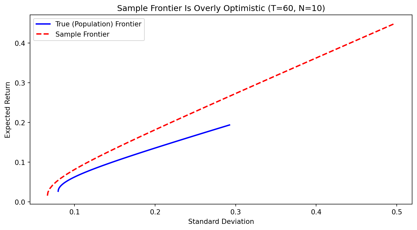
The sample frontier (red dashed) lies above and to the left of the true frontier (blue solid)—it promises higher returns for less risk, but this is an illusion.

Out-of-Sample Performance Is Worse

What happens when we invest based on the sample-optimal weights?

In-sample Sharpe ratios (what optimization promises) are much higher than out-of-sample Sharpe ratios (what we actually achieve).

The Effect of Sample Size and Dimensionality

The problem worsens as:

• Sample size (\(T\)) decreases: Less data means noisier estimates
• Number of assets (\(N\)) increases: More parameters to estimate, more opportunities for overfitting

When \(N\) is close to \(T\), the sample covariance matrix becomes nearly singular (hard to invert), and the sample-optimal weights become extreme and unstable.

This is exactly like overfitting in regression—too many parameters relative to the data.

How the Frontier Deteriorates

With more data (larger \(T\)), the sample frontier converges to the true frontier. With little data, the gap is substantial.

Part VI: Dealing with Estimation Risk

Approaches to Reduce Estimation Risk

Several strategies have been proposed:

1. Avoid optimization altogether: Use simple rules like equal weights (\(w_i = 1/N\))

2. Impose structure: Use factor models to reduce the number of parameters

3. Add constraints: Short-selling restrictions or bounds on weights

4. Target the minimum variance portfolio: It doesn’t depend on estimated expected returns

5. Combine portfolios optimally: Blend the tangency and minimum variance portfolios (Kan and Zhou, 2007)

6. Use regularization: Apply ML techniques like Lasso to shrink unstable weights

The 1/N Portfolio

The simplest approach: invest equally in all assets.

\[w_i = \frac{1}{N} \quad \text{for all } i\]

No estimation required!

DeMiguel, Garlappi, and Uppal (2009) compared 14 sophisticated portfolio optimization strategies to 1/N. Their finding:

None of the optimized portfolios consistently outperformed 1/N out of sample.

This is remarkable: decades of portfolio theory, and we often can’t beat naive diversification. The reason? Estimation error overwhelms the benefits of optimization.

The Global Minimum Variance Portfolio

Another robust option: the global minimum variance (GMV) portfolio — the portfolio with the lowest possible variance.

\[\mathbf{w}_{\text{GMV}} = \frac{\boldsymbol{\Sigma}^{-1} \mathbf{1}}{\mathbf{1}^\top \boldsymbol{\Sigma}^{-1} \mathbf{1}}\]

where \(\mathbf{1}\) is a vector of ones. This is the vertex of the efficient frontier — the leftmost point, where risk is minimized regardless of return.

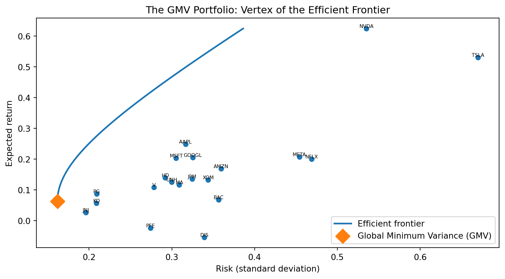
The GMV portfolio doesn’t depend on estimated expected returns — only on \(\boldsymbol{\Sigma}\). Since covariances are estimated more precisely than means, the GMV portfolio is more stable than the tangency portfolio.

From MVO to Regression

For a risk budget \(\sigma\), the mean-variance portfolio problem is:

\[\arg\max_{\mathbf{w}} \; \mathbf{w}^\top \boldsymbol{\mu} \quad \text{subject to} \quad \mathbf{w}^\top \boldsymbol{\Sigma} \mathbf{w} \leq \sigma^2\]

The explicit solution is \(\mathbf{w}^* = \frac{\sigma}{\sqrt{\theta}} \boldsymbol{\Sigma}^{-1} \boldsymbol{\mu}\), which requires inverting \(\hat{\boldsymbol{\Sigma}}\) — unstable when \(N\) is large relative to \(T\). It can be shown (we skip the derivation) that the quantity \(\boldsymbol{\mu}^\top \boldsymbol{\Sigma}^{-1} \boldsymbol{\mu}\) is the squared Sharpe ratio of the optimal (tangency) portfolio in MVO. Call it \(\theta\).

Ao, Li, and Zheng (2019, Review of Financial Studies) prove that this constrained optimization is equivalent to an unconstrained regression:

\[\mathbf{w}^* = \arg\min_{\mathbf{w}} \; E\left[(r_c - \mathbf{w}^\top \mathbf{r})^2\right], \quad \text{where } r_c = \sigma \frac{1 + \theta}{\sqrt{\theta}}\]

This avoids the matrix inversion entirely and opens the door to Lasso regularization.

MAXSER: Estimating \(r_c\) and Running Lasso

The regression on the previous slide requires \(r_c = \sigma \frac{1 + \theta}{\sqrt{\theta}}\), which depends on \(\theta = \boldsymbol{\mu}^\top \boldsymbol{\Sigma}^{-1} \boldsymbol{\mu}\) — the thing we’re trying to estimate in the first place. So we need an estimate \(\hat{\theta}\).

The plug-in (sample) estimate is:

\[\hat{\theta}_s = \hat{\boldsymbol{\mu}}^\top \hat{\boldsymbol{\Sigma}}^{-1} \hat{\boldsymbol{\mu}}\]

But \(\hat{\theta}_s\) is heavily biased upward when \(N/T\) isn’t negligible — the same estimation-risk problem from earlier in this lecture. So we use the bias-corrected estimator from Kan and Zhou (2007):

\[\hat{\theta} = \frac{(T - N - 2)\,\hat{\theta}_s - N}{T}\]

Ao et al. use a further adjusted version \(\theta_{\text{adj}}\) (their equation 1.32) to ensure \(\hat{\theta}\) stays non-negative. Once you have \(\hat{\theta}\), you compute \(\hat{r}_c\) and run Lasso:

\[\hat{\mathbf{w}}_{\text{MAXSER}} = \arg\min_{\mathbf{w}} \frac{1}{T} \sum_{t=1}^{T} (\hat{r}_c - \mathbf{w}^\top \mathbf{r}_t)^2 + \lambda \|\mathbf{w}\|_1\]

This is MAXSER — Maximum Sharpe Ratio Estimated by Sparse Regression. Cross-validation picks \(\lambda\), just like in standard Lasso.

Note that computing \(\hat{\theta}_s\) still requires \(\hat{\boldsymbol{\Sigma}}^{-1}\) — but only to produce a single scalar, not \(N\) portfolio weights. In plug-in MVO, the noisy inverse fans out into \(N\) unstable weight estimates. Here, the errors collapse into one number whose bias is well-characterized and correctable (the Kan–Zhou formula). Once you have \(\hat{r}_c\), the actual weight estimation is pure Lasso on raw returns — no inverse needed. The matrix inverse is quarantined to estimating a correctable scalar rather than directly determining all \(N\) weights.

You’ll implement this in Lab Report 4.

What MAXSER Gives You

MAXSER estimates a single portfolio: the tangency portfolio — the risky-asset portfolio with the highest Sharpe ratio. Recall that once you have the tangency, every investor just mixes it with the risk-free asset along the CAL. Risk aversion \(\gamma\) determines how far along the line you go. So estimating the tangency well is the whole game.

Plug-in tangency (\(\hat{\boldsymbol{\Sigma}}^{-1}\hat{\boldsymbol{\mu}}\), normalized) — uses all \(N\) assets with wildly unstable weights. High in-sample Sharpe, but this is overfitting: the optimizer exploits sample noise. Out of sample, the portfolio disappoints.

MAXSER tangency (Lasso regression with bias-corrected \(\hat{r}_c\), normalized) — sets most weights to exactly zero, invests in a sparse subset. Remaining weights are shrunk, preventing extreme positions. Lower in-sample Sharpe (honestly so), but more stable and often better out of sample.

This is overfitting vs. regularization — the same trade-off from Week 5, now applied to portfolios. You’ll implement MAXSER and compare it to plug-in MVO in Lab Report 4.

Choosing the Regularization Parameter

How do we choose \(\lambda\)?

Option 1: Cross-validation to maximize out-of-sample Sharpe ratio

Option 2: Cross-validation to match a target risk level

Option 3: Use an adjusted estimator for the Sharpe ratio that corrects for bias

The cross-validation approach is exactly what we learned in Week 5:

1. Split data into folds
2. For each \(\lambda\), fit on training folds, evaluate on test fold
3. Choose \(\lambda\) that gives best out-of-sample performance

Summary of ML Solutions

Method	Advantages	Disadvantages
1/N	No estimation, simple	Ignores all information
GMV	Ignores noisy means	Suboptimal if means are predictable
Constraints	Intuitive bounds	Ad hoc, may over-constrain
MAXSER (Lasso)	Principled, sparse, stable	Requires tuning \(\lambda\)

The ML approach (MAXSER) provides a principled way to balance:

• Using information in the data (through estimation)
• Not overfitting (through regularization)

Summary and Preview

What We Learned Today

Mean-variance utility provides a framework for ranking portfolios based on expected return and risk.

Optimal portfolios maximize utility, but the formulas require knowing true parameters \(\boldsymbol{\mu}\) and \(\boldsymbol{\Sigma}\).

Estimation risk arises because we must estimate parameters from limited data. This creates:

• Uncertainty in optimal weights
• Utility loss compared to the theoretical optimum
• Overly optimistic sample efficient frontiers

The curse of dimensionality: Utility loss grows linearly with the number of assets \(N\).

The ML Connection

This week showed that portfolio optimization is essentially a prediction problem:

• We’re predicting which assets will perform well
• Overfitting (to historical patterns) is a major concern
• Regularization techniques from ML help control overfitting

The MAXSER approach directly applies Lasso regression to portfolio construction, demonstrating that ML isn’t just for prediction—it’s also for decision-making under uncertainty.

This theme—using ML to improve financial decisions—continues throughout the course.

Next Week

Week 7: Linear Classification

We move from predicting continuous outcomes (regression) to predicting categories:

• Is a firm likely to default? (yes/no)
• Will the market go up or down? (up/down)
• What sector does a company belong to?

Classification is another core supervised learning problem with many applications in finance.

References

• Ao, M., Li, Y., & Zheng, X. (2019). Approaching mean-variance efficiency for large portfolios. Review of Financial Studies, 32(7), 2890-2919.
• DeMiguel, V., Garlappi, L., & Uppal, R. (2009). Optimal versus naive diversification: How inefficient is the 1/N portfolio strategy? Review of Financial Studies, 22(5), 1915-1953.
• Goyal, A., & Welch, I. (2008). A comprehensive look at the empirical performance of equity premium prediction. Review of Financial Studies, 21(4), 1455-1508.
• Kan, R., & Smith, D. R. (2008). The distribution of the sample minimum-variance frontier. Management Science, 54(7), 1364-1380.
• Kan, R., & Zhou, G. (2007). Optimal portfolio choice with parameter uncertainty. Journal of Financial and Quantitative Analysis, 42(3), 621-656.
• Markowitz, H. (1952). Portfolio selection. Journal of Finance, 7(1), 77-91.