RSM338: Machine Learning in Finance
Week 5: Regression | February 4–5, 2026
Kevin Mott
Rotman School of Management
Today’s Goal
You already know OLS from your statistics and econometrics courses. Today we build on that foundation.
The question: OLS works well under certain assumptions. What happens when those assumptions don’t hold—and what can we do about it?
Today’s roadmap:
- OLS as our starting point: The optimization perspective on what you already know
- When OLS struggles: Many predictors, multicollinearity, overfitting
- Generalizing OLS: Relaxing linearity, the loss function, and adding regularization
- In-sample vs out-of-sample: The core ML concern
- Bias-variance trade-off: Why more complex isn’t always better
- Regularization in practice: Ridge, Lasso, and Elastic Net
- Model selection: Cross-validation and choosing \(\lambda\)
- Finance applications: OOS R², why prediction is hard, common pitfalls
Part I: OLS as Our Starting Point
The OLS Framework You Know
From your statistics courses, you’ve seen the linear regression model:
\[\mathbf{y} = \mathbf{X}\boldsymbol{\beta} + \boldsymbol{\varepsilon}\]
OLS is an optimization problem. We choose \(\hat{\boldsymbol{\beta}}\) to minimize the residual sum of squares:
\[\hat{\boldsymbol{\beta}}^{\text{OLS}} = \arg\min_{\boldsymbol{\beta}} \sum_{i=1}^{n} (y_i - \mathbf{x}_i^\top \boldsymbol{\beta})^2 = \arg\min_{\boldsymbol{\beta}} \|\mathbf{y} - \mathbf{X}\boldsymbol{\beta}\|^2\]
The notation \(\|\mathbf{v}\|^2\) is the squared norm of vector \(\mathbf{v}\)—the sum of its squared elements:
\[\|\mathbf{v}\|^2 = v_1^2 + v_2^2 + \cdots + v_n^2 = \sum_{i=1}^{n} v_i^2\]
So \(\|\mathbf{y} - \mathbf{X}\boldsymbol{\beta}\|^2\) is just compact notation for \(\sum_{i=1}^{n} (y_i - \hat{y}_i)^2\).
This optimization problem has a closed-form solution:
\[\hat{\boldsymbol{\beta}}^{\text{OLS}} = (\mathbf{X}^\top \mathbf{X})^{-1} \mathbf{X}^\top \mathbf{y}\]
The argmin formulation makes explicit what OLS is doing: searching over all possible coefficient vectors \(\boldsymbol{\beta}\) and selecting the one that minimizes squared errors.
Why We Like OLS
OLS is the workhorse of statistics and econometrics for good reasons:
Simple and interpretable: Each coefficient \(\beta_j\) tells you how much \(Y\) changes when \(X_j\) increases by one unit, holding other variables constant.
Comes with standard errors: We can test whether coefficients are statistically significant (t-tests, p-values) and build confidence intervals.
Closed-form solution: No iterative algorithms needed—just matrix algebra.
In your statistics courses, OLS is typically used for inference: Is there a significant relationship between \(X\) and \(Y\)? How large is the effect?
When Does OLS Work Well?
OLS gives reliable estimates and valid hypothesis tests when certain conditions hold.
Linearity: The true relationship between \(X\) and \(Y\) is approximately linear.
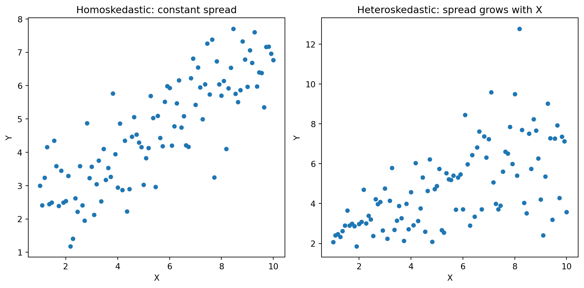
Homoskedasticity: The spread of errors is constant across all values of \(X\). “Homo” = same, “skedastic” = scatter.
No multicollinearity: Predictors should not be too highly correlated with each other.
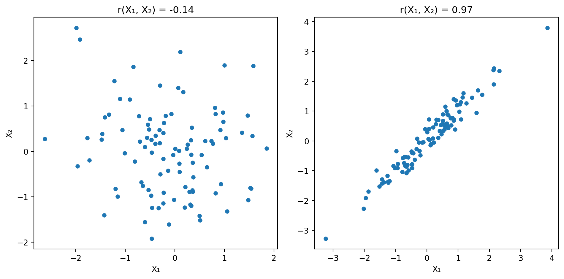
When predictors are highly correlated, \(\mathbf{X}^\top \mathbf{X}\) becomes nearly singular—hard to invert. Recall: \(\hat{\boldsymbol{\beta}} = (\mathbf{X}^\top \mathbf{X})^{-1} \mathbf{X}^\top \mathbf{y}\). Small changes in the data cause large swings in \(\hat{\boldsymbol{\beta}}\).
The ML Perspective: A Different Goal
Machine learning asks a different question: How well can we predict new data?
We care less about:
- Whether \(\beta_j\) is “significant”
- The “true” value of \(\beta_j\)
- Confidence intervals for effects
We care more about:
- Prediction accuracy on data we haven’t seen
- Whether the model generalizes beyond the training sample
- Balancing model complexity against overfitting
This shift in focus—from inference to prediction—changes what we optimize for.
Same Tool, Different Lens
Consider predicting next month’s stock returns from firm characteristics.
Econometrics lens:
- Does book-to-market ratio significantly predict returns?
- What is the estimated effect of a 1-unit change in B/M?
- Are the results robust to different specifications?
ML lens:
- If I train on 2000–2015 data, how well do I predict 2016–2020 returns?
- Does adding more predictors help or hurt out-of-sample?
- What’s the optimal amount of model complexity?
Both lenses use regression. But they emphasize different aspects.
Part II: What Can Go Wrong with OLS?
When OLS Struggles
OLS is a workhorse, but it has limitations—especially for prediction:
1. Many predictors relative to observations
When \(p\) (number of predictors) is large relative to \(n\) (observations), OLS estimates become unstable. In the extreme case where \(p > n\), OLS doesn’t even have a unique solution.
2. Multicollinearity
When predictors are highly correlated, \((\mathbf{X}^\top \mathbf{X})\) is nearly singular. Small changes in the data lead to large swings in coefficient estimates.
3. Overfitting
OLS uses all predictors, even those that add noise rather than signal. The model fits the training data too well—including its random noise—and generalizes poorly.
OLS in Finance: A Cautionary Tale
Suppose you want to predict monthly stock returns using firm characteristics.
You have \(n = 500\) firm-months and \(p = 50\) characteristics: size, book-to-market, momentum, volatility, industry dummies, and so on. With OLS:
- You estimate 51 parameters (50 betas plus intercept)
- Each coefficient has estimation error
- Many characteristics might be noise, not signal
- The fitted model explains the historical data well—but does it predict future returns?
Goyal and Welch (2008) examined this question in a seminal study. They tested whether classic predictors (dividend yield, earnings yield, book-to-market, etc.) could forecast the equity premium.
The finding: variables that appeared to predict returns historically often failed completely when used to predict future returns. Many predictors performed worse than simply guessing the historical average.
This isn’t a failure of the predictors per se—it’s a failure of OLS to generalize when signal is weak relative to noise.
Why Does This Happen?
OLS minimizes in-sample error. When the true signal is weak:
- OLS fits the noise in the training data
- This noise doesn’t appear in the same form in new data
- The noise-fitting hurts rather than helps prediction
The coefficients are unbiased in expectation—but they have high variance. When you apply them out-of-sample, the variance dominates.
This is the heart of the bias-variance trade-off we’ll formalize later.
Part III: Relaxing the OLS Framework
Three Ways to Generalize OLS
OLS makes specific choices that we can relax:
1. The functional form (linearity)
OLS assumes predictions are linear in \(X\). We could allow non-linear relationships.
2. The loss function (how we measure errors)
OLS minimizes squared error. We could minimize absolute error, or something else entirely.
3. Constraints on coefficients (regularization)
OLS places no constraints on \(\beta\). We could penalize large coefficients.
Relaxing Linearity: Where Does \(\mathbf{X}\boldsymbol{\beta}\) Come From?
Recall the OLS objective:
\[\hat{\boldsymbol{\beta}} = \arg\min_{\boldsymbol{\beta}} \sum_{i=1}^{n} (y_i - \mathbf{x}_i^\top \boldsymbol{\beta})^2\]
The term \(\mathbf{x}_i^\top \boldsymbol{\beta}\) is our prediction for observation \(i\). This assumes the prediction is a linear combination of the features:
\[\hat{y}_i = \beta_0 + \beta_1 x_{i1} + \beta_2 x_{i2} + \cdots + \beta_p x_{ip}\]
But nothing forces us to use a linear function. We could replace \(\mathbf{x}_i^\top \boldsymbol{\beta}\) with any function \(f(\mathbf{x}_i)\):
\[\hat{\theta} = \arg\min_{\theta} \sum_{i=1}^{n} (y_i - f_\theta(\mathbf{x}_i))^2\]
where \(f_\theta\) could be a polynomial, a tree, a neural network, or any other function parameterized by \(\theta\). We’ll explore non-linear \(f\) in later weeks (trees, neural networks).
Relaxing the Loss Function
OLS minimizes squared error. But why squared?
\[\mathcal{L}(\boldsymbol{\beta}) = \sum_{i=1}^{n} (y_i - \hat{y}_i)^2\]
Squared error is convenient (calculus gives a closed-form solution) and optimal under Gaussian errors. But it’s not the only choice.
Absolute error (L1 loss): \(\mathcal{L}(\boldsymbol{\beta}) = \sum_{i=1}^{n} |y_i - \hat{y}_i|\)
- Less sensitive to outliers than squared error
- No closed-form solution; requires iterative optimization
Huber loss: Squared for small errors, linear for large errors
- Combines robustness to outliers with smoothness near zero
The loss function \(\mathcal{L}\) defines what “good prediction” means. Choose it to match your goals.
Regularization: The Main Idea
Instead of just minimizing the loss, we add a penalty on coefficient size:
\[\text{minimize } \underbrace{\sum_{i=1}^{n} (y_i - \hat{y}_i)^2}_{\text{fit to data}} + \underbrace{\lambda \cdot \text{Penalty}(\boldsymbol{\beta})}_{\text{complexity cost}}\]
The parameter \(\lambda\) controls the trade-off:
- \(\lambda = 0\): No penalty, we get OLS
- \(\lambda \to \infty\): Heavy penalty, coefficients shrink to zero
Regularization deliberately introduces bias (coefficients are shrunk toward zero) in exchange for lower variance (more stable estimates).
When signal is weak relative to noise, this trade-off can improve prediction.
Measuring Size: The \(L_p\) Norm
A norm measures the “size” or “length” of a vector. The \(L_p\) norm is defined as:
\[\|\mathbf{v}\|_p = \left( \sum_{i=1}^{n} |v_i|^p \right)^{1/p}\]
Different values of \(p\) give different ways to measure length:
\(L_2\) norm (Euclidean): \(\|\mathbf{v}\|_2 = \sqrt{v_1^2 + v_2^2 + \cdots + v_n^2}\)
This is the familiar distance formula from the Pythagorean theorem. It’s the default notion of “length.”
\(L_1\) norm (Manhattan): \(\|\mathbf{v}\|_1 = |v_1| + |v_2| + \cdots + |v_n|\)
Sum of absolute values. Called “Manhattan” because it’s like walking along a grid of city blocks.
Two Types of Penalties
Now we can define our regularization penalties using norms:
Ridge regression (L2 penalty): Penalize the squared L2 norm of coefficients
\[\text{Penalty}(\boldsymbol{\beta}) = \|\boldsymbol{\beta}\|_2^2 = \sum_{j=1}^{p} \beta_j^2\]
Lasso regression (L1 penalty): Penalize the L1 norm of coefficients
\[\text{Penalty}(\boldsymbol{\beta}) = \|\boldsymbol{\beta}\|_1 = \sum_{j=1}^{p} |\beta_j|\]
Both penalties measure the “size” of the coefficient vector, but in different ways. This difference in geometry leads to very different behavior.
The General Regression Framework
We’ve seen three ways to generalize OLS. We can combine any or all of them:
\[\hat{\theta} = \arg\min_{\theta} \left\{ \underbrace{\sum_{i=1}^{n} \mathcal{L}(y_i, f_\theta(\mathbf{x}_i))}_{\text{loss function}} + \underbrace{\lambda \cdot \text{Penalty}(\theta)}_{\text{regularization}} \right\}\]
Choose your ingredients:
| Component | OLS Choice | Alternatives |
|---|---|---|
| Function \(f_\theta\) | Linear: \(\mathbf{x}^\top \boldsymbol{\beta}\) | Polynomial, tree, neural network |
| Loss \(\mathcal{L}\) | Squared error | Absolute error, Huber, quantile |
| Penalty | None (\(\lambda = 0\)) | Ridge (L2), Lasso (L1), Elastic Net |
This is the regression toolkit. Different combinations suit different problems. Today we focus on linear \(f\) with regularization; non-linear \(f\) comes in later weeks.
Part IV: In-Sample vs Out-of-Sample
The Core ML Concern
When we fit a model, we want to know: How well will it predict new data?
Training error (in-sample): How well does the model fit the data used to estimate it?
Test error (out-of-sample): How well does the model predict data it hasn’t seen?
A model’s training error is almost always an optimistic estimate of its true predictive ability.
Why? The model has been specifically tuned to the training data. Of course it does well there.
Overfitting: Setup
Overfitting occurs when a model learns the noise in the training data rather than the underlying pattern.
To illustrate, we’ll use polynomial regression. Instead of fitting a line \(f(x) = \beta_0 + \beta_1 x\), we fit a polynomial of degree \(d\):
\[f(x) = \beta_0 + \beta_1 x + \beta_2 x^2 + \cdots + \beta_d x^d\]
Higher degree = more flexible curve = more parameters to estimate.
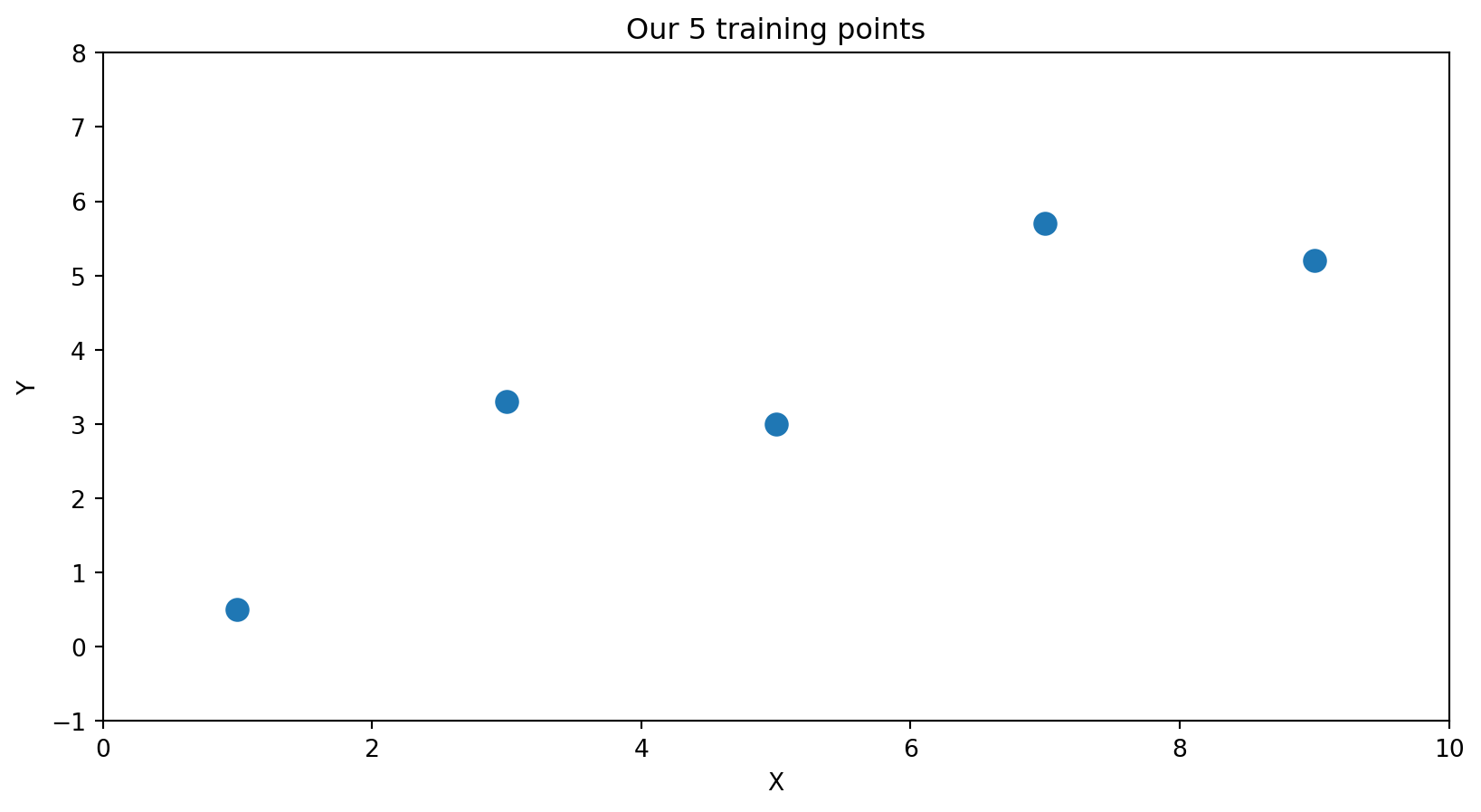
Suppose we have just 5 data points and the true relationship is linear (with noise):
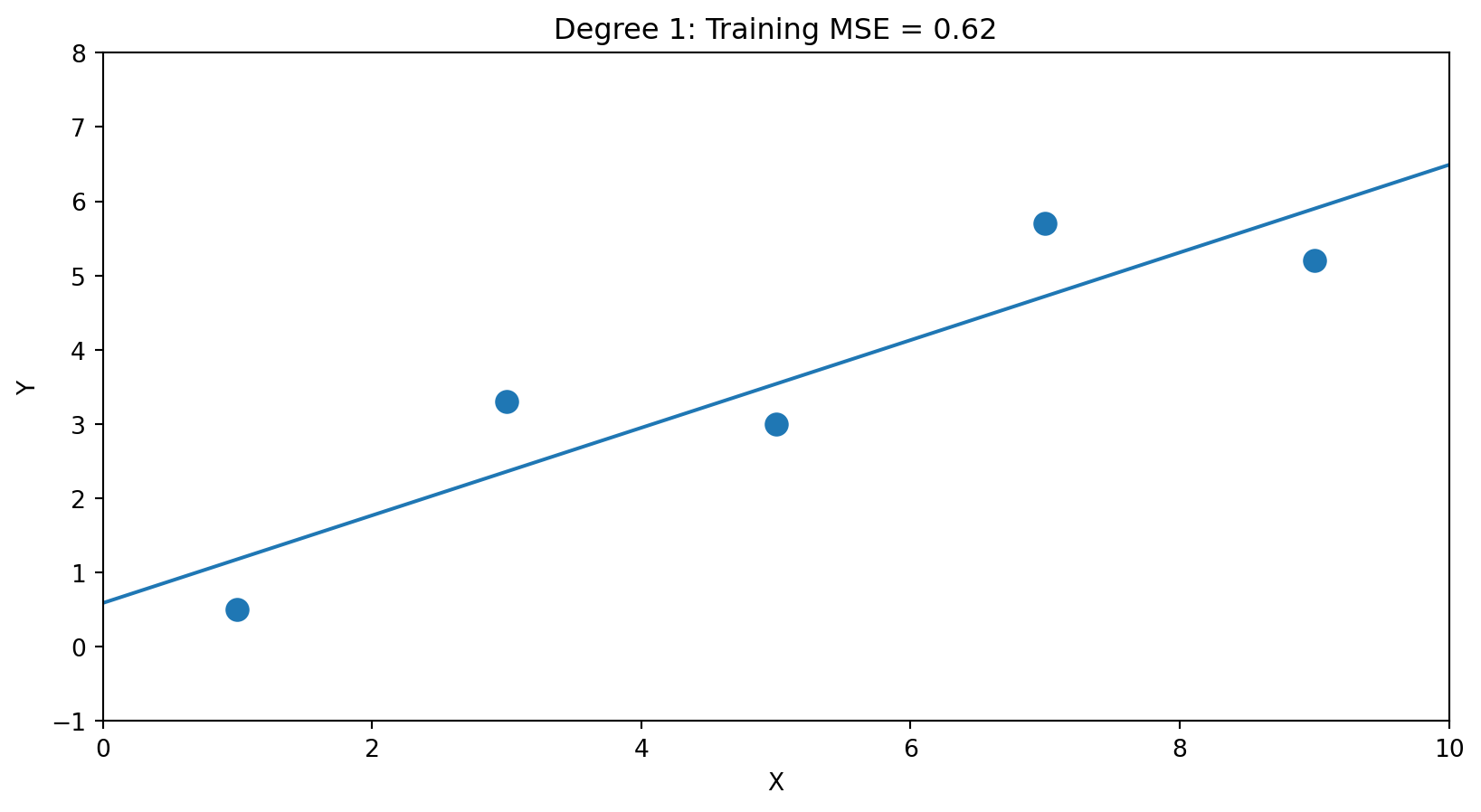
Degree 1 (2 parameters): \(\hat{f}(x) = \hat{\beta}_0 + \hat{\beta}_1 x\)
Degree 2 (3 parameters): \(\hat{f}(x) = \hat{\beta}_0 + \hat{\beta}_1 x + \hat{\beta}_2 x^2\)
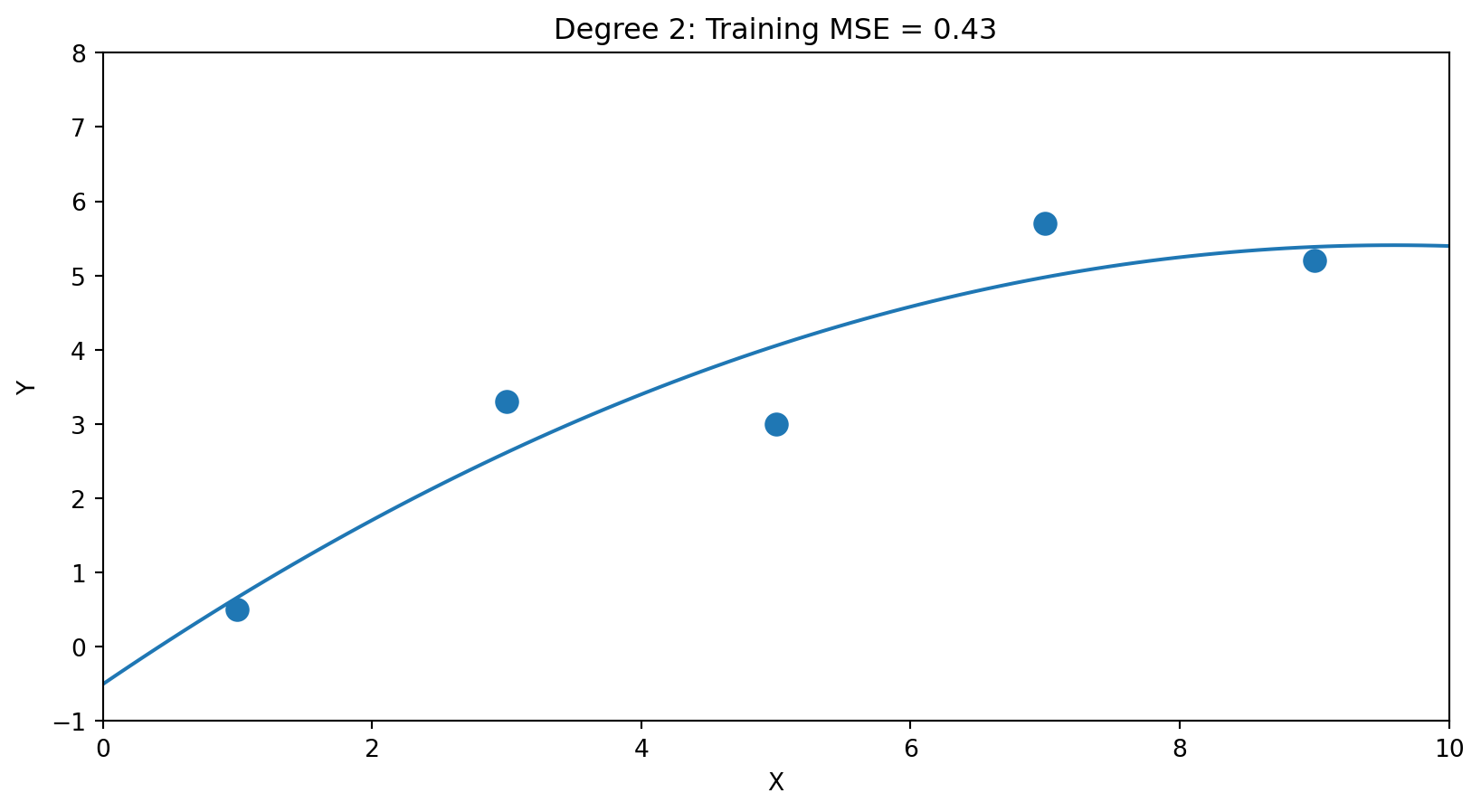
Degree 4 (5 parameters): \(\hat{f}(x) = \hat{\beta}_0 + \hat{\beta}_1 x + \cdots + \hat{\beta}_4 x^4\)
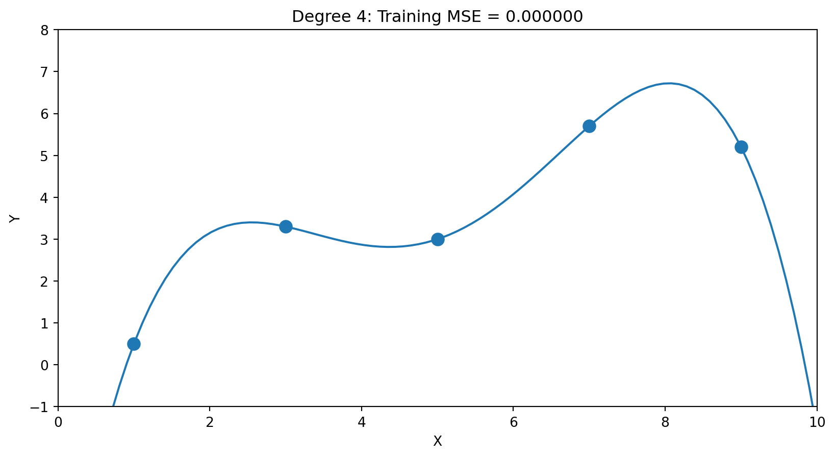
5 parameters for 5 points → perfect fit (MSE ≈ 0). But the wiggles are fitting noise, not signal.
And consider extrapolation: if we predict just slightly beyond \(X = 9\) (our last training point), this polynomial plummets—even though the data clearly suggests \(Y\) increases with \(X\). Overfit models can give wildly wrong predictions for interpolating or extrapolating.
The Problem: Training Error Always Falls
With enough parameters, we can fit the training data perfectly. But perfect fit ≠ good predictions.
| Degree | Parameters | Training MSE |
|---|---|---|
| 1 | 2 | Higher |
| 2 | 3 | Lower |
| 4 | 5 | ≈ 0 |
With enough parameters, we can fit the training data perfectly. But perfect training fit ≠ good predictions.
The model with zero training error has learned the noise specific to these 5 points. On new data, those wiggles will hurt, not help.
This is the fundamental tension: more complexity reduces training error but may increase test error.
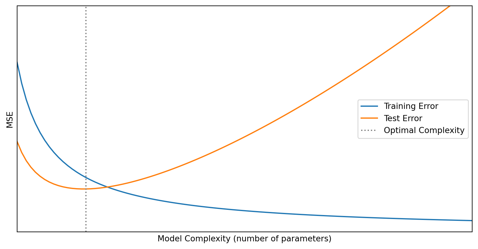
Training Error Always Falls; Test Error Doesn’t
As model complexity increases:
- Training error always decreases (more flexibility to fit the data)
- Test error first decreases, then increases (eventually we fit noise)
The Train-Test Split
The standard approach to evaluate predictive models:
- Split your data into training and test sets
- Fit the model using only the training data
- Evaluate using only the test data
The test data acts as a “held-out” check on how well the model generalizes.
from sklearn.model_selection import train_test_split
from sklearn.linear_model import LinearRegression
import numpy as np

# Generate data
np.random.seed(42)
X = np.random.randn(100, 5)  # 100 observations, 5 features
y = X[:, 0] + 0.5 * X[:, 1] + np.random.randn(100) * 0.5

# Split: 80% train, 20% test
X_train, X_test, y_train, y_test = train_test_split(X, y, test_size=0.2, random_state=42)

# Fit on training data only
model = LinearRegression()
model.fit(X_train, y_train)

# Evaluate on test data
train_mse = np.mean((y_train - model.predict(X_train))**2)
test_mse = np.mean((y_test - model.predict(X_test))**2)

print(f"Training MSE: {train_mse:.4f}")
print(f"Test MSE: {test_mse:.4f}")
Training MSE: 0.1967
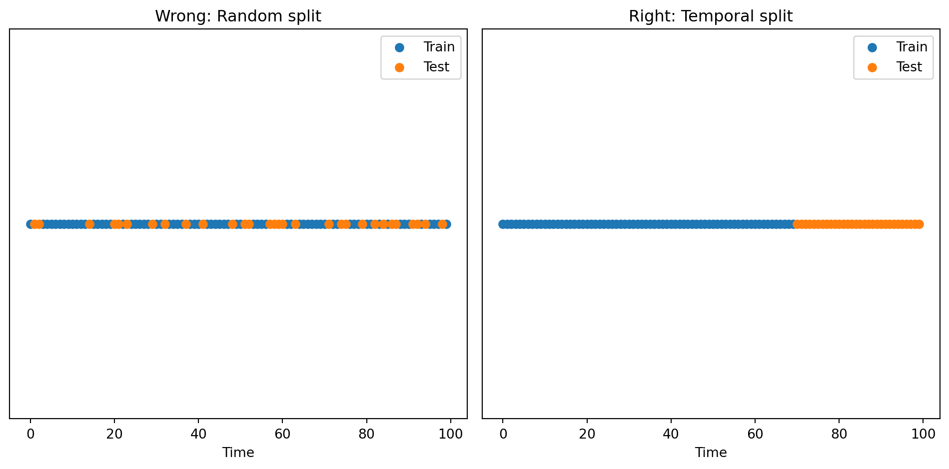
Test MSE: 0.2522Time Series: A Special Case
In finance, some data has a time dimension. We cannot randomly shuffle observations.
Wrong: Random train-test split allows future information to leak into training.
Right: Use a temporal split. Train on past data, test on future data.
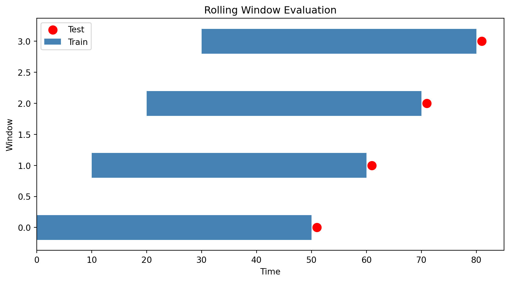
Rolling Windows for Time Series
For time series, a common approach is rolling window evaluation:
- Train on data from time 1 to \(T\)
- Predict time \(T+1\)
- Move the window: train on time 2 to \(T+1\)
- Predict time \(T+2\)
- Repeat…
This simulates what an investor would experience: making predictions using only past data.
Part V: The Bias-Variance Trade-off
Two Sources of Prediction Error
When a model makes prediction errors, there are two distinct sources:
Bias: Error from overly simplistic assumptions.
- A model with high bias “misses” the true pattern
- It systematically under- or over-predicts
- Think: fitting a constant when the true relationship is linear
Variance: Error from sensitivity to training data.
- A model with high variance is “unstable”
- Small changes in training data lead to very different predictions
- Think: a high-degree polynomial that wiggles through every training point
The Dartboard Analogy
Imagine throwing darts at a target, where the bullseye is the true value:
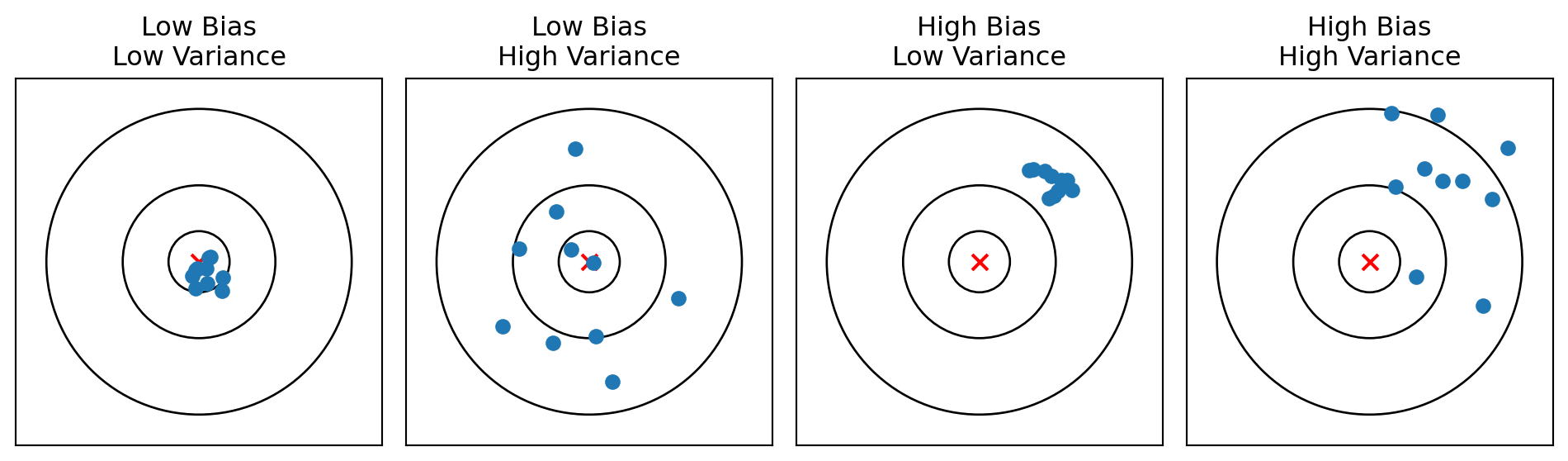
- Low bias, low variance: Predictions cluster tightly around the truth (ideal)
- High variance: Predictions are scattered (unstable)
- High bias: Predictions systematically miss the target
The Mathematical Decomposition
For a given test point, we can decompose the expected prediction error:
\[\mathbb{E}\left[(y - \hat{y})^2\right] = \text{Bias}^2 + \text{Variance} + \sigma^2\]
where:
- Bias² measures how far off the average prediction is from the truth
- Variance measures how much predictions vary across different training sets
- σ² is the irreducible noise in the data
Total error is the sum of these three terms. We can’t reduce \(\sigma^2\)—that’s the inherent randomness in the outcome.
The Trade-off
Reducing bias typically increases variance, and vice versa.
Simple models (few parameters):
- High bias (may miss patterns)
- Low variance (stable across training sets)
- Example: predicting returns with just the market factor
Complex models (many parameters):
- Low bias (can capture intricate patterns)
- High variance (sensitive to training data quirks)
- Example: regression with 50 firm characteristics
The optimal model balances these two sources of error.
Visualizing the Trade-off
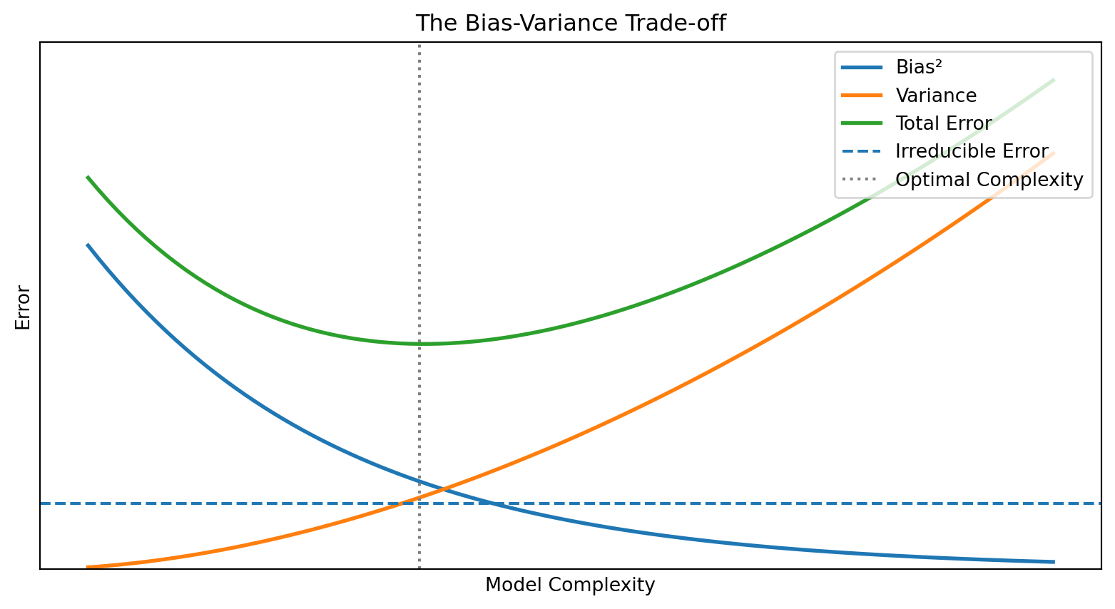
As complexity increases: bias falls, variance rises. Total error is U-shaped.
A Wrinkle: Double Descent
The classical picture says test error is U-shaped. But recent research discovered something surprising: if you keep increasing complexity past the interpolation threshold (where training error hits zero), test error can start decreasing again.
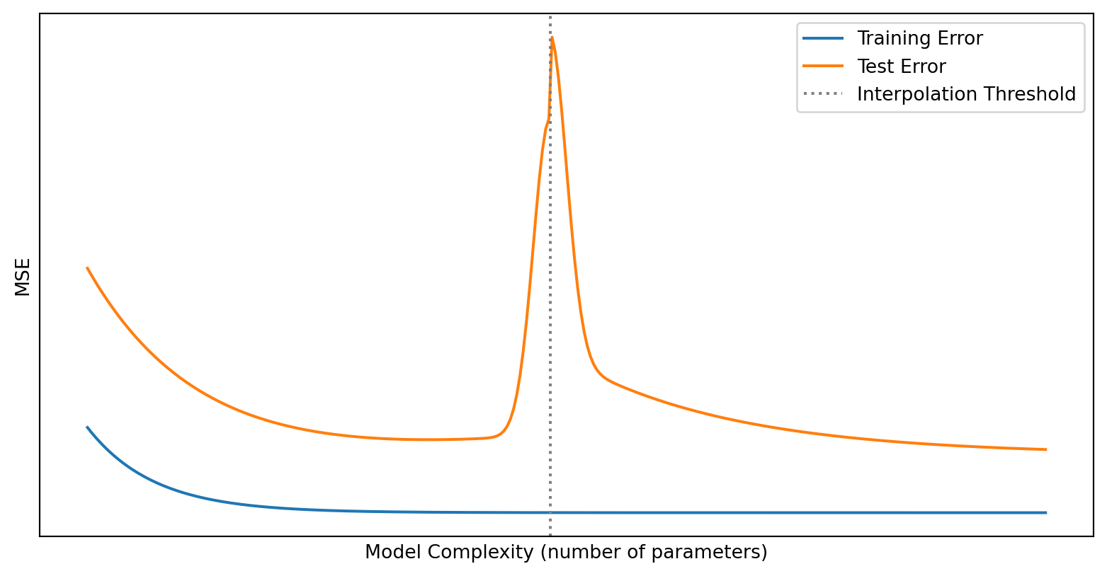
This is double descent (Belkin et al., 2019). It’s been observed in deep neural networks and other highly overparameterized models.
For this course, the classical U-shaped picture is the right mental model. But be aware that the story is more nuanced for very large models—an active area of research.
For an accessible explanation, see this excellent YouTube video: What the Books Get Wrong about AI [Double Descent]
Underfitting vs Overfitting
Underfitting (too simple):
- High bias, low variance
- Model doesn’t capture the true relationship
- Both training error and test error are high
Overfitting (too complex):
- Low bias, high variance
- Model fits noise in training data
- Training error is low, but test error is high
Just right:
- Balanced bias and variance
- Both training and test error are reasonably low
OLS and the Bias-Variance Trade-off
Where does OLS sit in this trade-off?
OLS is unbiased—in expectation, \(\mathbb{E}[\hat{\beta}] = \beta\) (under the standard assumptions).
But being unbiased doesn’t mean OLS minimizes prediction error. When:
- The true signal is weak
- You have many predictors
- Predictors are correlated
…OLS estimates have high variance. The variance component of prediction error dominates.
Regularization deliberately introduces bias to reduce variance. For prediction, this trade-off often improves total error.
Part VI: Regularization
Ridge Regression (L2 Penalty)
Ridge regression adds a penalty on the sum of squared coefficients:
\[\hat{\boldsymbol{\beta}}^{\text{ridge}} = \arg\min_{\boldsymbol{\beta}} \left\{ \sum_{i=1}^{n} (y_i - \mathbf{x}_i^\top \boldsymbol{\beta})^2 + \lambda \sum_{j=1}^{p} \beta_j^2 \right\}\]
In matrix form:
\[\hat{\boldsymbol{\beta}}^{\text{ridge}} = \arg\min_{\boldsymbol{\beta}} \left\{ \|\mathbf{y} - \mathbf{X}\boldsymbol{\beta}\|^2 + \lambda \|\boldsymbol{\beta}\|_2^2 \right\}\]
This has a closed-form solution:
\[\hat{\boldsymbol{\beta}}^{\text{ridge}} = (\mathbf{X}^\top \mathbf{X} + \lambda \mathbf{I})^{-1} \mathbf{X}^\top \mathbf{y}\]
The term \(\lambda \mathbf{I}\) adds \(\lambda\) to the diagonal of \(\mathbf{X}^\top \mathbf{X}\), making it invertible even when OLS would fail.
Ridge Regression: Properties
What does ridge regression do?
- Shrinks all coefficients toward zero, but never sets them exactly to zero
- Handles multicollinearity by stabilizing the matrix inversion
- Reduces variance at the cost of introducing bias
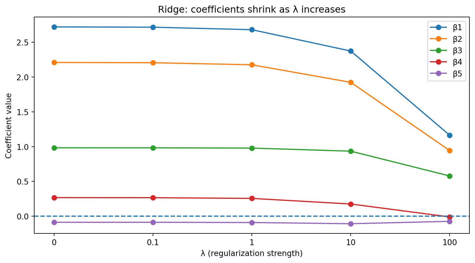
As \(\lambda\) increases, coefficients shrink toward zero but never reach exactly zero.
Lasso Regression (L1 Penalty)
Lasso (Least Absolute Shrinkage and Selection Operator) penalizes the sum of absolute coefficients:
\[\hat{\boldsymbol{\beta}}^{\text{lasso}} = \arg\min_{\boldsymbol{\beta}} \left\{ \sum_{i=1}^{n} (y_i - \mathbf{x}_i^\top \boldsymbol{\beta})^2 + \lambda \sum_{j=1}^{p} |\beta_j| \right\}\]
Unlike ridge, lasso can set coefficients exactly to zero.
This means lasso performs variable selection—it automatically identifies which predictors matter and which don’t.
There’s no closed-form solution; lasso requires iterative optimization algorithms.
Lasso: Properties
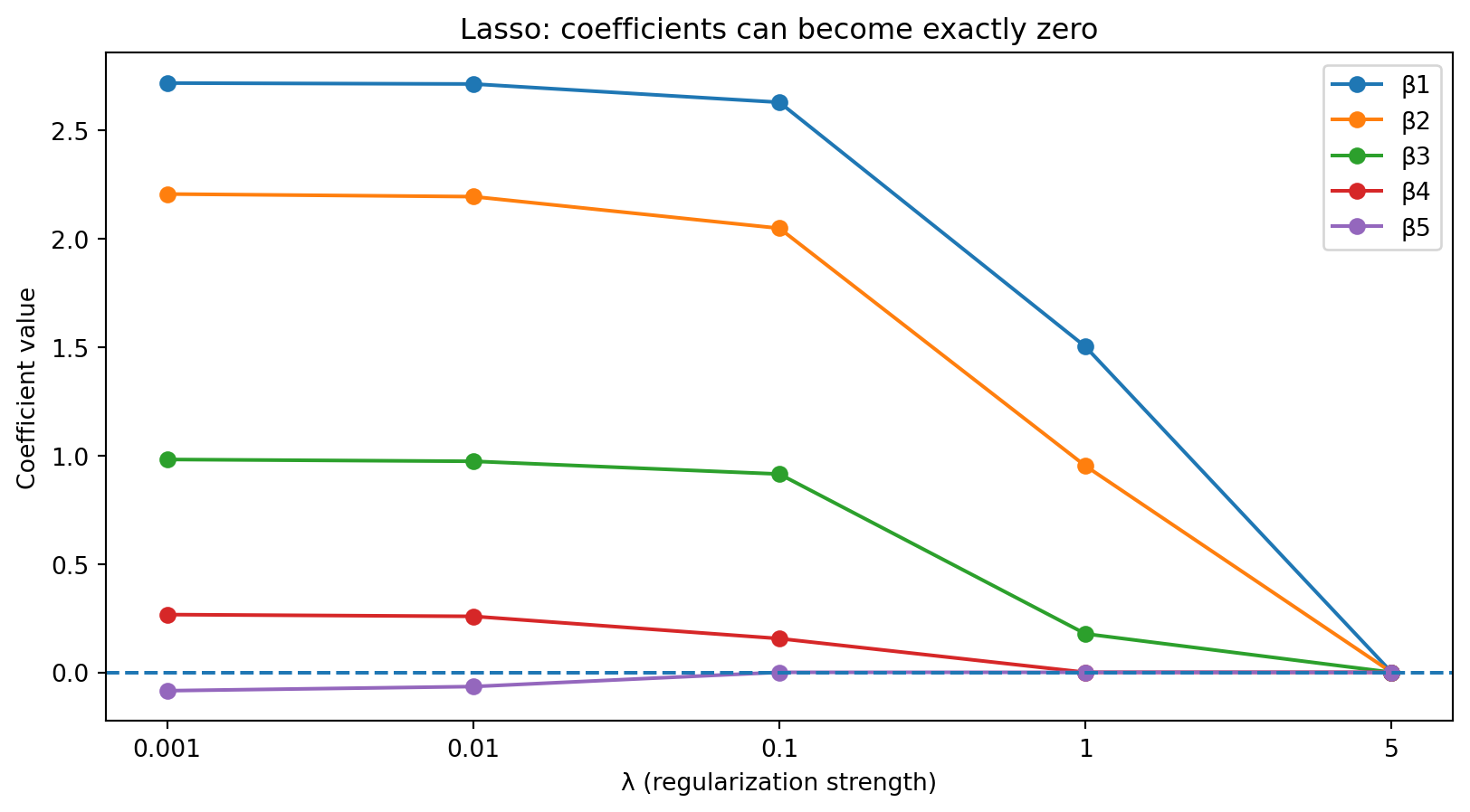
As \(\lambda\) increases, some coefficients hit exactly zero—those predictors are dropped from the model.
Ridge vs Lasso: When to Use Which?
Use Ridge when:
- You believe most predictors have some effect
- Predictors are correlated (multicollinearity)
- You want stable coefficient estimates
Use Lasso when:
- You believe only a few predictors matter (sparse model)
- You want automatic variable selection
- Interpretability is a priority
In practice, try both and let cross-validation decide.
Elastic Net: Combining Ridge and Lasso
Elastic Net combines L1 and L2 penalties:
\[\hat{\boldsymbol{\beta}}^{\text{EN}} = \arg\min_{\boldsymbol{\beta}} \left\{ \|\mathbf{y} - \mathbf{X}\boldsymbol{\beta}\|^2 + \lambda \left[ \alpha \|\boldsymbol{\beta}\|_1 + (1-\alpha) \|\boldsymbol{\beta}\|_2^2 \right] \right\}\]
The parameter \(\alpha\) controls the mix:
- \(\alpha = 1\): Pure Lasso
- \(\alpha = 0\): Pure Ridge
- \(0 < \alpha < 1\): A combination
Elastic Net is useful when you want variable selection (like Lasso) but predictors are correlated (where Lasso can be unstable).
Regularization in Python
from sklearn.linear_model import Ridge, Lasso, ElasticNet
from sklearn.preprocessing import StandardScaler

# Generate data with sparse true coefficients
np.random.seed(42)
n, p = 100, 10
X = np.random.randn(n, p)
true_beta = np.array([2, 1, 0.5, 0, 0, 0, 0, 0, 0, 0])
y = X @ true_beta + np.random.randn(n) * 0.5

# Standardize features (required for regularization)
scaler = StandardScaler()
X_scaled = scaler.fit_transform(X)

# Fit models
ols = LinearRegression().fit(X_scaled, y)
ridge = Ridge(alpha=1.0).fit(X_scaled, y)
lasso = Lasso(alpha=0.1).fit(X_scaled, y)
enet = ElasticNet(alpha=0.1, l1_ratio=0.5).fit(X_scaled, y)

print("True coefficients: [2, 1, 0.5, 0, 0, 0, 0, 0, 0, 0]")
print(f"OLS:    {np.round(ols.coef_, 2)}")
print(f"Ridge:  {np.round(ridge.coef_, 2)}")
print(f"Lasso:  {np.round(lasso.coef_, 2)}")
print(f"ElNet:  {np.round(enet.coef_, 2)}")
True coefficients: [2, 1, 0.5, 0, 0, 0, 0, 0, 0, 0]
OLS: [ 1.74 1.01 0.5 0.01 -0.07 0.03 -0.09 -0. 0.02 -0.03]
Ridge: [ 1.72 1. 0.5 0.01 -0.07 0.03 -0.09 -0. 0.02 -0.04]
Lasso: [ 1.65 0.92 0.4 -0. -0. 0. -0.01 -0. -0. -0. ]
ElNet: [ 1.61 0.91 0.43 0. -0. 0. -0.06 0. 0. -0.01]Standardization Matters
Before applying regularization, always standardize your features.
Why? The penalty treats all coefficients equally. If features are on different scales, the penalty affects them unequally.
Example: If \(X_1\) is market cap (values in billions) and \(X_2\) is book-to-market ratio (values around 0.5), the coefficient on \(X_1\) will naturally be tiny. Without standardization, it barely gets penalized while \(X_2\) gets penalized heavily.
Standardization: subtract the mean and divide by the standard deviation for each feature:
\[z_j = \frac{x_j - \bar{x}_j}{s_j}\]
After standardization, all features have mean 0 and standard deviation 1. The penalty affects them equally.
Part VII: Model Selection and Cross-Validation
The Model Selection Problem
We need to choose:
- Which predictors to include (or let Lasso decide)
- How much regularization (\(\lambda\))
- Which type of model (Ridge, Lasso, Elastic Net, etc.)
The goal: find the model that generalizes best to new data.
We can’t use training error—it always favors more complex models.
We can’t use all our data for testing—we need data to train the model.
Solution: cross-validation.
K-Fold Cross-Validation
K-fold cross-validation estimates test error without wasting data:
- Split the data into \(K\) equal-sized “folds”
- For each fold \(k = 1, \ldots, K\):
- Use fold \(k\) as the validation set
- Use all other folds as the training set
- Fit the model and compute validation error
- Average the \(K\) validation errors
This gives a more robust estimate of test error than a single train-test split.
Common choices: \(K = 5\) or \(K = 10\).
Cross-Validation: Visualized
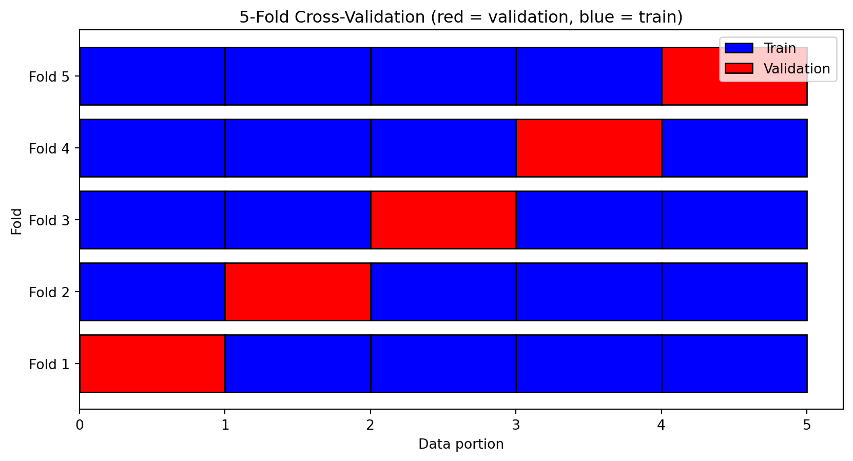
Each data point is used for validation exactly once. We get 5 estimates of test error and average them.
Choosing \(\lambda\) with Cross-Validation
from sklearn.model_selection import cross_val_score
from sklearn.linear_model import Lasso

# Generate data
np.random.seed(42)
X = np.random.randn(200, 10)
y = 2*X[:, 0] + X[:, 1] + 0.5*X[:, 2] + np.random.randn(200)*0.5

# Try different lambda values
lambdas = [0.001, 0.01, 0.1, 0.5, 1.0]
cv_scores = []

for lam in lambdas:
    model = Lasso(alpha=lam)
    # 5-fold CV, negative MSE (sklearn uses negative for "higher is better" convention)
    scores = cross_val_score(model, X, y, cv=5, scoring='neg_mean_squared_error')
    cv_scores.append(-scores.mean())

print("Lambda\tCV MSE")
for lam, score in zip(lambdas, cv_scores):
    print(f"{lam}\t{score:.4f}")

print(f"\nBest lambda: {lambdas[np.argmin(cv_scores)]}")
Lambda CV MSE
0.001 0.2581
0.01 0.2550
0.1 0.2725
0.5 0.9950
1.0 2.6882
Best lambda: 0.01Built-in Cross-Validation
sklearn provides LassoCV and RidgeCV that automatically find the best \(\lambda\):
from sklearn.linear_model import LassoCV

# LassoCV automatically searches over lambda values
lasso_cv = LassoCV(cv=5, random_state=42)
lasso_cv.fit(X, y)

print(f"Best lambda: {lasso_cv.alpha_:.4f}")
print(f"Non-zero coefficients: {np.sum(lasso_cv.coef_ != 0)} out of 10")
print(f"Coefficients: {np.round(lasso_cv.coef_, 3)}")
Best lambda: 0.0231
Non-zero coefficients: 8 out of 10
Coefficients: [ 1.988 1.028 0.43 0.025 0. -0.016 -0.019 -0.017 -0. 0.029]Time Series Cross-Validation
For time series, standard K-fold CV is inappropriate—it randomly mixes past and future.
Use TimeSeriesSplit which always trains on past, validates on future:
from sklearn.model_selection import TimeSeriesSplit

# TimeSeriesSplit with 5 folds
X_ts = np.arange(20).reshape(-1, 1)
tscv = TimeSeriesSplit(n_splits=5)

print("TimeSeriesSplit folds:")
for i, (train_idx, test_idx) in enumerate(tscv.split(X_ts)):
    print(f"Fold {i+1}: Train {train_idx[0]}-{train_idx[-1]}, Test {test_idx[0]}-{test_idx[-1]}")
TimeSeriesSplit folds:
Fold 1: Train 0-4, Test 5-7
Fold 2: Train 0-7, Test 8-10
Fold 3: Train 0-10, Test 11-13
Fold 4: Train 0-13, Test 14-16
Fold 5: Train 0-16, Test 17-19The training set expands with each fold, respecting the temporal order.
Part VIII: Finance Applications
Out-of-Sample R²: The Finance Metric
In finance, we evaluate predictive regressions using out-of-sample R²:
\[R^2_{OOS} = 1 - \frac{\sum_{t=1}^{T} (r_t - \hat{r}_t)^2}{\sum_{t=1}^{T} (r_t - \bar{r})^2}\]
where:
- \(r_t\) is the actual return at time \(t\)
- \(\hat{r}_t\) is the predicted return (using only information before time \(t\))
- \(\bar{r}\) is the historical mean return (the “naive” forecast)
Interpretation:
- \(R^2_{OOS} > 0\): Model beats predicting the historical mean
- \(R^2_{OOS} = 0\): Model performs same as historical mean
- \(R^2_{OOS} < 0\): Model is worse than just predicting the mean
Computing OOS R² in Python
def oos_r_squared(y_actual, y_predicted, y_mean_benchmark):
    """
    Compute out-of-sample R-squared.

    y_actual: actual returns
    y_predicted: model predictions
    y_mean_benchmark: historical mean predictions
    """
    ss_model = np.sum((y_actual - y_predicted)**2)
    ss_benchmark = np.sum((y_actual - y_mean_benchmark)**2)
    return 1 - ss_model / ss_benchmark

# Example: model that adds noise to actual returns
np.random.seed(42)
y_actual = np.random.randn(100) * 0.02  # Simulated monthly returns
y_predicted = y_actual + np.random.randn(100) * 0.03  # Noisy predictions
y_benchmark = np.full(100, y_actual.mean())

r2_oos = oos_r_squared(y_actual, y_predicted, y_benchmark)
print(f"OOS R²: {r2_oos:.4f}")
OOS R²: -1.4825Negative OOS R² is common in return prediction—the model is worse than the naive mean.
Why Is Return Prediction So Hard?
Several factors make financial returns difficult to predict:
Low signal-to-noise ratio: The predictable component of returns is tiny compared to the unpredictable component. Monthly stock return volatility is ~5%; any predictable component is a fraction of that.
Non-stationarity: Relationships change over time. A predictor that worked in the 1980s may not work today.
Competition: Markets are full of smart participants. Easy predictability gets arbitraged away.
Estimation error: Even if a relationship exists, estimating it precisely requires more data than we have.
Campbell and Thompson (2008) show that even an OOS R² of 0.5% has economic value—but achieving even that is hard.
Common Pitfalls in Financial ML
Look-ahead bias: Using information that wouldn’t have been available at prediction time.
- Example: Using December earnings to predict January returns, when earnings aren’t reported until March
Survivorship bias: Only including firms that survived to the present.
- Excludes bankruptcies, delistings, acquisitions
- Typically makes strategies look better than reality
Data snooping: Trying many predictors and reporting only those that “work.”
- If you test 100 predictors at 5% significance, expect 5 false positives
- Harvey, Liu, and Zhu (2016) argue t-statistics should exceed 3.0, not 2.0
Transaction costs: A predictor may be statistically significant but economically unprofitable.
Regularization in Return Prediction
Regularization is particularly valuable in finance because:
- Many potential predictors: Factor zoo has hundreds of proposed characteristics
- Weak signals: True predictability is small; OLS overfits noise
- Multicollinearity: Many characteristics are correlated (size and book-to-market, momentum and volatility)
- Panel structure: With stocks × months, \(n\) is large but so is \(p\)
Studies like Gu, Kelly, and Xiu (2020) show that regularized methods (especially Lasso and Elastic Net) outperform OLS for predicting stock returns out-of-sample.
A Finance Checklist
Before trusting any regression result:
Data quality:
- Does the data include delisted/bankrupt firms? (survivorship bias)
- Are variables measured as of the prediction date? (look-ahead bias)
Evaluation:
- Is performance measured out-of-sample?
- Is the OOS R² positive?
- For time series: is the split temporal, not random?
Statistical validity:
- How many predictors were tried? (data snooping)
- Are standard errors appropriate? (clustering, panel structure)
Economic significance:
- Is the strategy profitable after costs?
- Is the sample period representative?
Summary
OLS as optimization: \(\hat{\boldsymbol{\beta}}^{\text{OLS}} = \arg\min_{\boldsymbol{\beta}} \|\mathbf{y} - \mathbf{X}\boldsymbol{\beta}\|^2\). It’s unbiased, but can have high variance when signal is weak or predictors are many/correlated.
Generalizing OLS: We can relax the functional form (\(f\) doesn’t have to be linear), the loss function (doesn’t have to be squared error), and add regularization (penalize coefficient size).
In-sample vs out-of-sample: Training error always falls with complexity; test error doesn’t. This is why we evaluate on held-out data.
Bias-variance trade-off: Simple models have high bias/low variance; complex models have low bias/high variance. Total error is minimized at intermediate complexity. (Though double descent shows this isn’t the whole story for very large models.)
Regularization: Ridge (L2) shrinks all coefficients; Lasso (L1) can set coefficients exactly to zero. Elastic Net combines both. Always standardize features first.
Cross-validation estimates out-of-sample performance and helps choose \(\lambda\). For time series, use temporal splits.
In finance: Prediction is hard (low signal-to-noise, non-stationarity, competition). Use OOS R², watch for look-ahead bias, survivorship bias, and data snooping.
Next Week
Week 6: ML and Portfolio Theory
How do we use predicted returns to construct portfolios?
- Mean-variance optimization with estimated inputs
- The curse of estimation error
- Regularized portfolio construction
References
- Campbell, J. Y., & Thompson, S. B. (2008). Predicting excess stock returns out of sample: Can anything beat the historical average? Review of Financial Studies, 21(4), 1509-1531.
- Goyal, A., & Welch, I. (2008). A comprehensive look at the empirical performance of equity premium prediction. Review of Financial Studies, 21(4), 1455-1508.
- Gu, S., Kelly, B., & Xiu, D. (2020). Empirical asset pricing via machine learning. Review of Financial Studies, 33(5), 2223-2273.
- Harvey, C. R., Liu, Y., & Zhu, H. (2016). …and the cross-section of expected returns. Review of Financial Studies, 29(1), 5-68.
- Hastie, T., Tibshirani, R., & Friedman, J. (2009). The Elements of Statistical Learning (2nd ed.). Springer. Chapters 3 and 7.
- Hull, J. (2024). Machine Learning in Business: An Introduction to the World of Data Science (3rd ed.). Chapters 3-4.
- James, G., Witten, D., Hastie, T., & Tibshirani, R. (2021). An Introduction to Statistical Learning (2nd ed.). Springer. Chapters 5-6.