RSM338: Applications of Machine Learning in Finance
Week 3: Introduction to Machine Learning | January 21–22, 2026
Kevin Mott
Rotman School of Management
Today’s Roadmap
Last week, we studied the statistical properties of financial returns—how they’re distributed, why the normality assumption fails, and why prediction is hard. Today we step back to understand the broader framework: Machine Learning.
- What is Machine Learning? Learning patterns from data
- Types of Learning: Supervised, unsupervised, and reinforcement learning
- The ML Formalism: Loss functions, parameters, and learning algorithms
- Python for ML: The tools you’ll use and how to read code
- Limitations: When ML fails and why
Part I: What is Machine Learning?
The Traditional Programming Approach
Traditional programming: You write explicit rules for the computer to follow.
Example: Building a spam filter the traditional way:
IF email contains "Nigerian prince" THEN spam
IF email contains "free money" THEN spam
IF sender is in contacts THEN not spam
IF email contains "urgent wire transfer" THEN spam
...
Problems with this approach:
- You must anticipate every possible pattern
- Rules become unwieldy as edge cases accumulate
- The world changes—new spam tactics appear constantly
- Some patterns are too complex for humans to articulate
Question: How would you write rules to recognize a cat in a photo? Or predict tomorrow’s stock return?
The Machine Learning Approach
Machine learning: Instead of writing rules, you show the computer examples and let it learn the patterns.
The same spam filter, ML approach:
- Collect thousands of emails labeled “spam” or “not spam”
- Feed them to an ML algorithm
- The algorithm learns which patterns distinguish spam from legitimate email
- Apply the learned patterns to new emails
For many problems, it’s easier to collect examples than to write rules.
Machine Learning = building models that learn patterns directly from data, rather than being explicitly programmed.
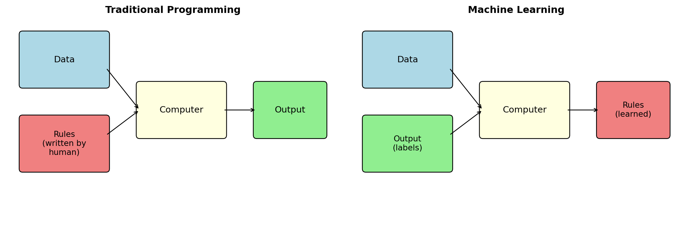
Traditional Programming vs. Machine Learning
Traditional programming: Human writes rules, computer applies them to data.
Machine learning: Human provides data and desired outputs, computer learns the rules.
Why Use Machine Learning?
Use ML when:
- Rules are too complex to articulate: Recognizing faces, understanding speech, reading handwriting
- Rules change over time: Fraud patterns evolve, market regimes shift
- Rules differ across contexts: What predicts returns varies by asset class, time period, market conditions
- You have lots of labeled examples: The data itself can reveal the patterns
Finance examples where ML excels:
- Credit scoring: Which borrowers will default? (millions of loan records)
- Fraud detection: Which transactions are fraudulent? (labeled fraud cases)
- Return prediction: Which stocks will outperform? (historical returns + features)
- Portfolio construction: How to group similar assets? (return patterns)
Connection to What We’ve Done
Week 2 set up the problem ML tries to solve:
- We have historical data (S&P 500 returns)
- We want to estimate parameters (\(\mu\), \(\sigma\)) and make forecasts (expected wealth)
- Estimation is uncertain—more data helps, but we’re never perfectly sure
- Most predictors fail out-of-sample (Goyal-Welch)
Machine learning is a systematic framework for:
- Choosing what to estimate (model selection)
- Measuring how wrong we are (loss functions)
- Finding the best estimates (learning algorithms)
- Testing whether our estimates generalize (out-of-sample evaluation)
Part II: Types of Learning
Three Types of Machine Learning
1. Supervised Learning
- You have labeled data: input-output pairs \((x_i, y_i)\)
- Goal: Learn a function \(f\) such that \(f(x) \approx y\)
- Examples: spam detection, return prediction, credit scoring
2. Unsupervised Learning
- You have only inputs \(x_i\)—no labels
- Goal: Discover structure or patterns in the data
- Examples: clustering stocks, dimensionality reduction, anomaly detection
3. Reinforcement Learning
- An agent learns by interacting with an environment
- Goal: Maximize cumulative reward through trial and error
- Examples: game playing, robotic control, trading strategies
This course focuses on supervised and unsupervised learning. We won’t cover reinforcement learning.
Building Your ML Toolbox
Think of ML methods as tools in a toolbox.
Just as an experienced contractor knows which tool is right for each repair—hammer for nails, wrench for bolts, saw for cutting—you’ll learn which ML method is right for each problem.
The tools we’ll cover:
| Tool | What it does | When to use it |
|---|---|---|
| Linear regression | Predict a number from features | Simple relationships, interpretability matters |
| Regularized regression | Prevent overfitting | Many features, small samples |
| Logistic regression | Predict probabilities/classes | Binary outcomes (default/no default) |
| Decision trees | Capture nonlinear patterns | Complex interactions between features |
| Clustering | Group similar observations | No labels, want to find structure |
The goal of this course: Build your intuition so you recognize which tool fits which problem—and understand why.
Supervised Learning: The Setup
The prediction problem:
Given input features \(\mathbf{x}\) (what we observe), predict an output \(y\) (what we want to know).
Notation:
- \(\mathbf{x}_i = (x_{i1}, x_{i2}, \ldots, x_{ip})'\) — a \(p\)-dimensional feature vector for observation \(i\)
- \(y_i\) — the target or label for observation \(i\)
- \(\mathcal{D} = \{(\mathbf{x}_1, y_1), (\mathbf{x}_2, y_2), \ldots, (\mathbf{x}_N, y_N)\}\) — the training set of \(N\) labeled examples
The goal: Learn a function \(f: \mathbb{R}^p \to \mathcal{Y}\) such that \(f(\mathbf{x}) \approx y\).
Two main types of supervised learning:
| Type | Target \(y\) | Example |
|---|---|---|
| Regression | Continuous (real-valued) | Predict stock return, house price |
| Classification | Categorical (discrete) | Predict spam/not spam, buy/sell/hold |
Regression vs. Classification
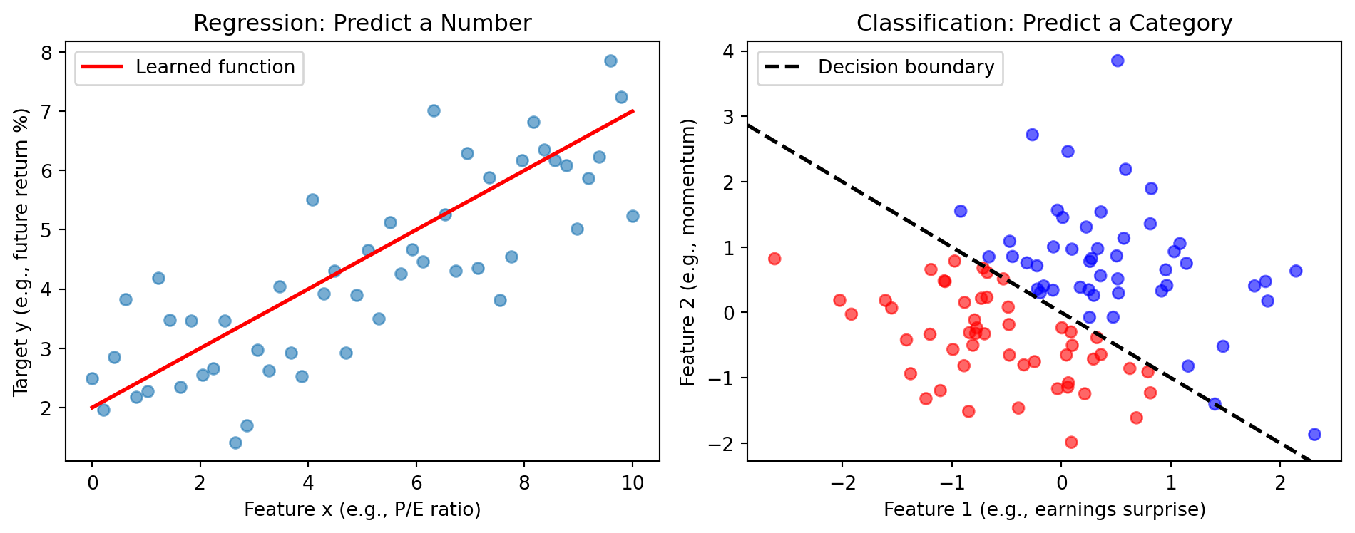
Regression: The target \(y\) is a continuous number. We want to minimize how far off our predictions are.
Classification: The target \(y\) is a category (class). We want to predict the correct class as often as possible.
Regression: Starting with Linear
Linear regression assumes the relationship between features and target is linear:
\[y = \beta_0 + \beta_1 x_1 + \beta_2 x_2 + \cdots + \beta_p x_p + \varepsilon\]
In matrix form, for \(N\) observations:
\[\mathbf{y} = \mathbf{X}\boldsymbol{\beta} + \boldsymbol{\varepsilon}\]
where \(\mathbf{y} \in \mathbb{R}^N\), \(\mathbf{X} \in \mathbb{R}^{N \times (p+1)}\), and \(\boldsymbol{\beta} \in \mathbb{R}^{p+1}\).
The OLS solution: \(\hat{\boldsymbol{\beta}} = (\mathbf{X}'\mathbf{X})^{-1}\mathbf{X}'\mathbf{y}\)
This is the “learning algorithm” for linear regression—it finds the \(\boldsymbol{\beta}\) that minimizes squared error.
Beyond Linearity: ML as Function Approximation
The ML perspective: We’re trying to approximate some unknown function \(f\):
\[y = f(\mathbf{x}) + \varepsilon\]
This function \(f\) could be linear: \(f(\mathbf{x}) = \mathbf{X}\boldsymbol{\beta}\). But it might not be.
We don’t know what \(f\) is. That’s what “learning” means—finding a good approximation \(\hat{f}\) from data, whether that turns out to be linear or not.
Different ML methods = different assumptions about \(f\):
| Method | Assumption about \(f\) |
|---|---|
| Linear regression | \(f\) is linear |
| Polynomial regression | \(f\) is a polynomial |
| Decision trees | \(f\) is piecewise constant |
| Deep neural networks | \(f\) is a composition of simple nonlinear functions: which can approximate any continuous function! |
The tradeoff: More flexible models can fit complex patterns, but risk overfitting (fitting noise instead of signal) and have growing computational costs.
Finance Examples: Classification
Credit scoring:
- Features \(\mathbf{x}\): Income, debt, credit history, employment, …
- Target \(y\): Default or No Default (binary classification)
Fraud detection:
- Features \(\mathbf{x}\): Transaction amount, time, location, merchant type, …
- Target \(y\): Fraudulent or Legitimate (binary)
Trading signals:
- Features \(\mathbf{x}\): Technical indicators, fundamentals, sentiment, …
- Target \(y\): Buy, Hold, or Sell (multi-class classification)
Ordinal classification (a hybrid):
- Target \(y\): Credit rating (AAA, AA, A, BBB, …) — categories with natural ordering
- Sometimes treated as regression, sometimes as classification
Unsupervised Learning: The Setup
The structure-discovery problem:
Given only input features \(\mathbf{x}\)—no labels—find interesting patterns or structure.
Notation:
- Data: \(\{\mathbf{x}_1, \mathbf{x}_2, \ldots, \mathbf{x}_N\}\) — just features, no labels
Key difference from supervised learning:
- Supervised: We ask “given features \(\mathbf{x}\), what is \(y\)?” — we model \(P(Y | \mathbf{X})\)
- Unsupervised: We ask “what does the data look like?” — we model \(P(\mathbf{X})\)
In supervised learning, there’s a target variable \(y\) we’re trying to predict. In unsupervised learning, there’s no \(y\)—we’re just trying to understand the structure of \(\mathbf{X}\) itself. Which observations are similar? Are there natural groupings? What are the main patterns?
Main unsupervised tasks:
| Task | Goal | Example |
|---|---|---|
| Clustering | Group similar observations | Group stocks by return patterns |
| Dimensionality reduction | Find low-dimensional representation | Reduce 100 features to 5 factors |
| Density estimation | Estimate the data distribution | Model the joint distribution of returns |
| Anomaly detection | Find unusual observations | Detect outlier transactions |
Finance Examples: Unsupervised Learning
Clustering stocks:
- Group stocks that move together
- Identify “sectors” from return data (without using industry labels)
- Construct diversified portfolios by sampling from different clusters
Factor models / PCA:
- Find the dominant factors driving returns
- Reduce dimensionality from thousands of stocks to a few factors
- Recall from RSM332: Factor models decompose returns into systematic and idiosyncratic components
Anomaly detection:
- Identify unusual trading patterns
- Detect market manipulation
- Flag outlier returns for further investigation
We’ll study clustering (K-means) in detail in Week 4.
Reinforcement Learning: Brief Introduction
The sequential decision problem:
An agent interacts with an environment over time, receiving rewards or penalties for its actions.
The setup:
- State \(s_t\): Current situation (e.g., current portfolio, market conditions)
- Action \(a_t\): What the agent does (e.g., buy, sell, hold)
- Reward \(r_t\): Feedback from the environment (e.g., profit/loss)
- Goal: Learn a policy \(\pi(s) \to a\) that maximizes cumulative reward
Finance applications:
- Optimal execution (minimize market impact when trading large orders)
- Portfolio management (dynamic asset allocation)
- Market making (set bid-ask spreads)
Why it’s different:
- Actions affect future states (your trade moves the price)
- Delayed rewards (today’s trade affects tomorrow’s opportunities)
- Exploration vs. exploitation (try new strategies vs. stick with what works)
We won’t cover RL in depth, but it’s an active research area in quantitative finance.
Part III: The ML Formalism
The Three Ingredients of Machine Learning
Every ML algorithm has three components:
- A model: What functions \(f\) are we considering?
- A loss function: How do we measure prediction error?
- A learning algorithm: How do we find the best \(f\)?
Example: Linear regression
- Model: \(f(\mathbf{x}) = \beta_0 + \beta_1 x_1 + \cdots + \beta_p x_p\) (linear functions)
- Loss: Squared error \(L(y, \hat{y}) = (y - \hat{y})^2\)
- Algorithm: Ordinary least squares: \(\hat{\boldsymbol{\beta}} = (\mathbf{X}'\mathbf{X})^{-1}\mathbf{X}'\mathbf{y}\)
The ML framework gives us a systematic way to think about prediction problems.
Ingredient 1: The Model
The model is the function \(f(\mathbf{x})\) we’re trying to learn.
We have to decide what form \(f\) takes. This is a choice we make:
| Model type | Form | Parameters to learn |
|---|---|---|
| Linear regression | \(f(\mathbf{x}) = \beta_0 + \beta_1 x_1 + \cdots + \beta_p x_p\) | \(\boldsymbol{\beta}\) |
| Polynomial | \(f(x) = \beta_0 + \beta_1 x + \beta_2 x^2 + \cdots\) | Coefficients |
| Decision tree | Piecewise constant regions | Split points, leaf values |
| Neural network | Compositions of nonlinear functions | Weights and biases |
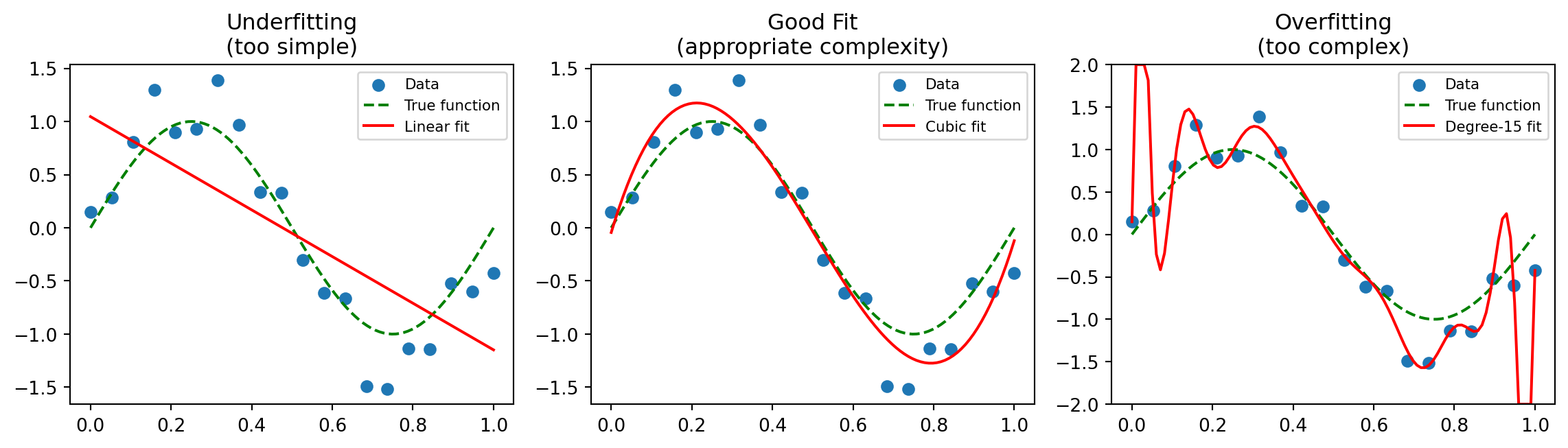
The tradeoff:
- Too simple a model: Can’t capture the true relationship (underfitting)
- Too complex a model: Fits noise in the training data (overfitting)
Learning = finding the parameters. Once we choose a model form (e.g., linear), the learning algorithm finds the specific parameter values (e.g., \(\hat{\boldsymbol{\beta}}\)) that best fit the data.
Ingredient 2: The Loss Function
The loss function measures how bad a prediction is.
Notation:
- \(L(y, \hat{y})\) = loss when true value is \(y\) and prediction is \(\hat{y}\)
- Lower loss = better prediction
Common loss functions for regression:
| Name | Formula | Properties |
|---|---|---|
| Squared error | \(L(y, \hat{y}) = (y - \hat{y})^2\) | Penalizes large errors heavily |
| Absolute error | \(L(y, \hat{y}) = |y - \hat{y}|\) | More robust to outliers |
Common loss functions for classification:
| Name | Formula | Properties |
|---|---|---|
| 0-1 loss | \(L(y, \hat{y}) = \mathbf{1}[y \neq \hat{y}]\) | 1 if wrong, 0 if correct |
| Cross-entropy | \(L(y, p) = -y \log p - (1-y)\log(1-p)\) | For probabilistic predictions |
The loss function defines what “good prediction” means.
Average Loss: The Objective Function
We want to minimize average loss across the training data.
Empirical risk (training error):
\[\mathcal{L}(\boldsymbol{\theta}) = \frac{1}{N} \sum_{i=1}^{N} L(y_i, f_{\boldsymbol{\theta}}(\mathbf{x}_i))\]
For squared error loss:
\[\mathcal{L}(\boldsymbol{\theta}) = \frac{1}{N} \sum_{i=1}^{N} (y_i - f_{\boldsymbol{\theta}}(\mathbf{x}_i))^2 = \text{MSE}\]
The learning problem becomes an optimization problem:
\[\boldsymbol{\theta}^* = \arg\min_{\boldsymbol{\theta}} \mathcal{L}(\boldsymbol{\theta})\]
Find the parameters \(\boldsymbol{\theta}^*\) that minimize average loss on the training data.
Ingredient 3: The Learning Algorithm
The learning algorithm finds the optimal parameters \(\boldsymbol{\theta}^*\).
For some problems, there’s a closed-form solution:
Linear regression with squared error:
\[\boldsymbol{\beta}^* = (\mathbf{X}'\mathbf{X})^{-1}\mathbf{X}'\mathbf{y}\]
This is the OLS formula from your statistics courses.
For most problems, we use iterative optimization:
Gradient descent: Move parameters in the direction that reduces loss.
\[\boldsymbol{\theta}^{(t+1)} = \boldsymbol{\theta}^{(t)} - \eta \nabla_{\boldsymbol{\theta}} \mathcal{L}(\boldsymbol{\theta}^{(t)})\]
where:
- \(\nabla_{\boldsymbol{\theta}} \mathcal{L}\) is the gradient (vector of partial derivatives)
- \(\eta > 0\) is the learning rate (step size)
- We iterate until convergence
Gradient descent is the workhorse of modern ML—it’s how neural networks are trained.
Why Derivatives? The Intuition
We want to minimize error. From calculus, you know that minima occur where the derivative equals zero:
\[\frac{d\mathcal{L}}{d\theta} = 0 \quad \Rightarrow \quad \theta^*\]
Problem: For complex models, we can’t solve this equation analytically.
Solution: Use the derivative to guide us toward the minimum.
The gradient \(\nabla \mathcal{L}\) points in the direction of steepest increase. So the negative gradient points toward steepest decrease.
\[\underbrace{-\nabla_{\boldsymbol{\theta}} \mathcal{L}}_{\text{direction of steepest decrease}}\]
Gradient descent: Take small steps in the direction of steepest decrease until we reach a point where \(\nabla \mathcal{L} \approx 0\) (a minimum).
This is like walking downhill in fog—you can’t see the bottom, but you can feel which direction is steepest and step that way.
Visualizing Gradient Descent
Gradient descent iteratively moves “downhill” on the loss surface until it reaches a minimum.
Putting It Together: The ML Recipe
Step 1: Choose a model
- What form should \(f\) take?
- Linear? Polynomial? Tree? Neural network?
Step 2: Choose a loss function
- How do we measure prediction quality?
- Squared error? Absolute error? Classification accuracy?
Step 3: Fit the model (run the learning algorithm)
- Find parameters \(\boldsymbol{\theta}^*\) that minimize training loss
- Use closed-form solution or gradient descent
Step 4: Evaluate on new data
- Training error is optimistic (overfitting risk)
- Test on held-out data (out-of-sample evaluation)—as we discussed in Week 2!
Part IV: Python for Machine Learning
The Python ML Ecosystem
You don’t need to be a programmer to use ML. Most of the hard work is already done—you just need to know which tools to use.
The main packages:
| Package | What it does | You’ll use it to… |
|---|---|---|
numpy |
Fast math on arrays | Store data, do matrix operations |
pandas |
Data tables (like Excel) | Load CSV files, clean data, compute returns |
matplotlib |
Plotting | Visualize results |
scikit-learn |
ML algorithms | Fit models, make predictions, evaluate |
All of these are pre-installed in most Python environments (Anaconda, Google Colab, etc.).
The Typical ML Workflow
The algorithms behind ML are genuinely complex—gradient descent, matrix decompositions, optimization routines. A production implementation of random forests is thousands of lines of code.
But Python is a language built on packages. Someone else has already:
- Written the complex algorithms
- Debugged edge cases
- Optimized for speed (often using C/Fortran under the hood)
So our code stays high-level and brief:
1. Load data         →  pandas.read_csv()
2. Prepare features  →  pandas/numpy operations
3. Split data        →  sklearn.model_selection.train_test_split()
4. Fit model         →  model.fit(X_train, y_train)
5. Make predictions  →  model.predict(X_test)
6. Evaluate          →  Compare predictions to truth
Every ML project follows this pattern. The hard work is understanding which model to use and how to interpret results—that’s what this course teaches.
Example: Complete ML Pipeline
import numpy as np
import pandas as pd
import matplotlib.pyplot as plt
from sklearn.linear_model import LinearRegression
from sklearn.model_selection import train_test_split

# 1. Create some fake stock data
np.random.seed(42)
data = pd.DataFrame({
    'market_return': np.random.randn(100),
    'stock_return': np.random.randn(100)
})
data['stock_return'] = 0.5 + 1.2 * data['market_return'] + 0.3 * np.random.randn(100)

# Visualize the raw data
plt.scatter(data['market_return'], data['stock_return'])
plt.xlabel('Market Return')
plt.ylabel('Stock Return')
plt.title('Step 1: Look at your data')
plt.show()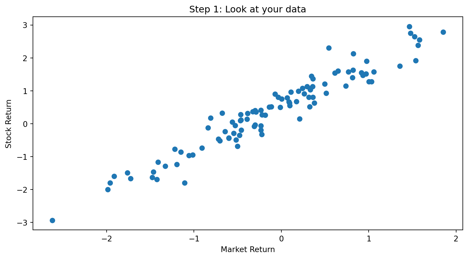
# 2. Split into training and test sets
X = data[['market_return']]  # Features (what we observe)
y = data['stock_return']      # Target (what we predict)
X_train, X_test, y_train, y_test = train_test_split(X, y, test_size=0.2)

# 3. Fit model
model = LinearRegression()
model.fit(X_train, y_train)

print(f"Estimated beta: {model.coef_[0]:.2f}")
print(f"Estimated alpha: {model.intercept_:.2f}")

# Visualize the fitted model
plt.scatter(X_train, y_train, label='Training data')
x_line = np.linspace(-3, 3, 100)
plt.plot(x_line, model.intercept_ + model.coef_[0] * x_line, color='red', label='Fitted line')
plt.xlabel('Market Return')
plt.ylabel('Stock Return')
plt.title('Step 2: Fit the model')
plt.legend()
plt.show()
Estimated beta: 1.28
Estimated alpha: 0.54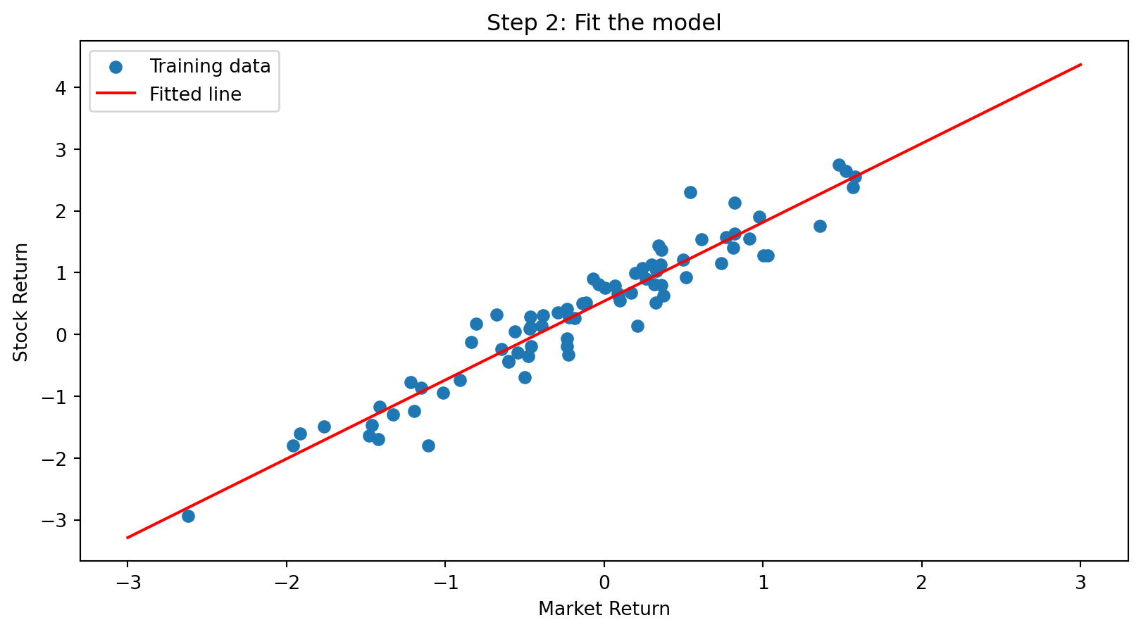
# 4. Predict on test data and evaluate
predictions = model.predict(X_test)

# Visualize: predicted vs actual
plt.scatter(y_test, predictions)
plt.plot([-2, 3], [-2, 3], 'r--', label='Perfect predictions')  # 45-degree line
plt.xlabel('Actual Stock Return')
plt.ylabel('Predicted Stock Return')
plt.title('Step 3: Evaluate predictions')
plt.legend()
plt.show()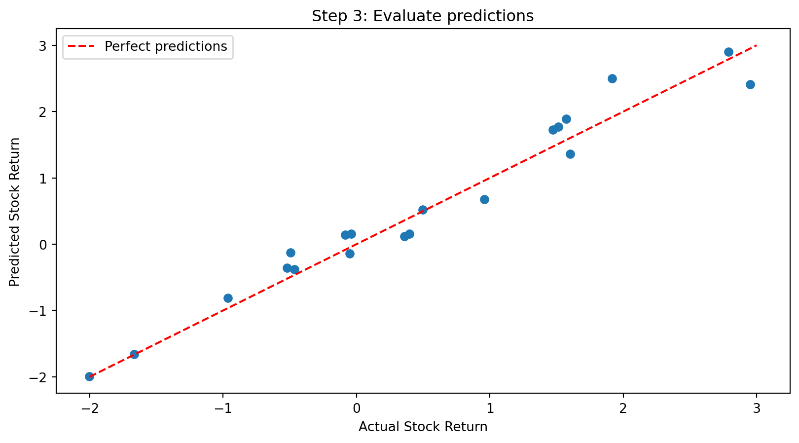
scikit-learn: The Workhorse
Almost every ML model in scikit-learn uses the same interface:
Swapping models is easy:
# Linear regression
from sklearn.linear_model import LinearRegression
model = LinearRegression()

# Ridge regression (with regularization)
from sklearn.linear_model import Ridge
model = Ridge(alpha=1.0)

# Random forest
from sklearn.ensemble import RandomForestRegressor
model = RandomForestRegressor()

# The rest of the code stays the same!
You learn one interface, you can use dozens of models.
Reading Code: What to Focus On
When you see code in this course, don’t panic. Focus on:
1. What data goes in?
2. What model are we using?
3. What comes out?
You don’t need to memorize syntax. You need to understand what the code is doing.
Common Patterns You’ll See
Loading data:
Computing log returns:
Selecting columns:
Train/test split:
These patterns repeat constantly. After a few weeks, they’ll feel natural.
Part V: Limitations and Summary
When Machine Learning Fails
ML is not magic. It fails when its assumptions are violated.
1. Dependence on historical data
- ML learns patterns from the past
- If the future differs systematically, predictions fail
- Finance example: A model trained on bull market data may fail in a crash
2. The stationarity assumption
- Most ML methods assume the data-generating process is stable
- If relationships change over time, models become stale
- Finance example: Factor returns vary across market regimes
3. Regime changes
- Major structural breaks invalidate learned patterns
- Examples: 2008 financial crisis, COVID-19 pandemic, regulatory changes
- In 2020, many demand forecasting models failed when consumption patterns changed overnight
Reality Check
“All models are wrong, but some are useful.” — George Box
Overfitting: The Central Challenge
Overfitting: The model learns noise in the training data rather than true patterns.
Symptoms:
- Excellent performance on training data
- Poor performance on new data (out-of-sample)
Prevention strategies (covered in later weeks):
- Cross-validation (evaluate on held-out data)
- Regularization (penalize model complexity)
- Early stopping (stop training before overfitting)
Overfitting: The Central Challenge
Week 2 previewed this: most return predictors fail out-of-sample (Goyal-Welch 2008). Why?
Overfitting: The model learns patterns in the training data that don’t generalize.
- Some patterns are real (signal)
- Some patterns are coincidence (noise)
- A model fit to historical data captures both
The ML terminology:
| Term | Meaning |
|---|---|
| Training error | Performance on data used to fit the model |
| Test error | Performance on new, unseen data |
| Overfitting | Training error << Test error |
Much of this course is about avoiding overfitting:
- Train/test splits (today’s Python examples)
- Regularization (Week 5)
- Cross-validation (Week 5)
- Ensemble methods (Week 9)
Today’s Key Takeaways
What is Machine Learning?
- Learning patterns from data rather than explicitly programming rules
- Three ingredients: model, loss function, learning algorithm
Types of Learning:
- Supervised: Labeled data → predict output from features
- Regression (continuous target) vs. Classification (categorical target)
- Unsupervised: No labels → discover structure
- Clustering, dimensionality reduction
- Reinforcement: Learn through interaction and rewards
The ML Formalism:
- Choose a model (what form should \(f\) take?)
- Define a loss function (how to measure error)
- Run a learning algorithm (find best parameters)
Python for ML:
- scikit-learn provides a consistent interface:
fit(),predict() - Same workflow for every model: load data → split → fit → predict → evaluate
- You don’t need to memorize syntax—focus on what the code is doing
Limitations:
- Overfitting is the central challenge; out-of-sample evaluation is essential
- ML depends on historical data—past patterns may not persist
What’s Next
| Week | Topic |
|---|---|
| 4 | Clustering |
| 5 | Regression (linear, ridge, lasso) |
| 6 | ML & Portfolio Theory |
| 7 | Linear Classification |
| 8 | Nonlinear Classification |
| 9 | Ensemble Methods |
| 10 | Neural Networks & Deep Learning |
| 11 | Text & NLP |
Each week adds new tools to your toolbox—and everything builds on the framework we introduced today.