RSM338: Applications of Machine Learning in Finance

Week 2: Financial Data | January 14–15, 2026

Kevin Mott

Rotman School of Management

Motivation and Overview

Much of quantitative finance—and the ML applications we will study—centers on return prediction.

  • We model and forecast returns because they have convenient statistical properties.

However, investors ultimately care about wealth: the dollar value of their portfolio.

  • Wealth is a nonlinear function of returns, which creates a fundamental issue.
  • In general, for a nonlinear function \(f\) and random variable \(X\): \[\mathbb{E}[f(X)] \neq f(\mathbb{E}[X])\]
  • As we will see, we usually choose to model log returns: \(r_t = \ln P_{t} - \ln P_{t-1}\)
  • A standard statistical assumption is that log returns \(r_t\) are normally distributed
  • Wealth is a function of returns: \(W_t = f(r_t)\)
  • What does this imply for the distribution of wealth \(W_t\)? \[ r_t \sim \mathcal N \implies W_t \sim \boxed{\quad\quad\quad} \text{?} \]

This means that knowing the expected return does not directly tell us the expected wealth.

Today’s Lecture

Today we develop the statistical framework for working with financial returns—from basic definitions through the challenges of prediction.

Part I: From Log Returns to Log-Normal Wealth

  • Why we use log returns and how they relate to wealth
  • If log returns are normal, wealth is log-normal
  • The “variance boost”: why expected wealth exceeds the naïve forecast

Part II: Estimation Risk

  • We estimate \(\mu\) from historical data—how does that uncertainty affect forecasts?
  • Estimation error introduces additional upward bias in wealth projections

Part III: Testing the Normality Assumption

  • Skewness and kurtosis: measuring deviations from normality
  • Empirical evidence: S&P 500 returns have fat tails (extreme events are far more common than normal predicts)

Part IV: Why Prediction Is Hard

  • Autocorrelation is tiny; most predictors fail out-of-sample
  • Preview: overfitting and the IS/OOS distinction

Part I: From Log Returns to Log-Normal Wealth

Simple (Arithmetic) Returns

The simple return (or arithmetic return) from period \(t-1\) to \(t\) is:

\[R_t = \frac{P_t + d_t}{P_{t-1}} - 1\]

where:

  • \(P_t\) = price at time \(t\)
  • \(P_{t-1}\) = price at time \(t-1\)
  • \(d_t\) = dividend paid during period (if any)

Example: If \(P_{t-1} = 100\), \(P_t = 105\), and \(d_t = 2\):

\[R_t = \frac{105 + 2}{100} - 1 = 0.07 \text{ or } 7\%\]

Interpretation: it tells you how much your wealth grew.

The Problem with Simple Returns: Compounding and Annualization

Suppose you earn \(R_1 = 10\%\) in year 1 and \(R_2 = 10\%\) in year 2.

What is your total return over both years?

Not \(10\% + 10\% = 20\%.\) Instead:

\[1 + R_{1\to2} = (1 + R_1)(1 + R_2) = (1.10)(1.10) = 1.21\]

So \(R_{1\to2} = 21\%.\)

Simple returns compound multiplicatively, not additively.

In general, over \(T\) years:

\[1 + R_{1 \to T} = (1 + R_1)(1 + R_2) \cdots (1 + R_T) = \prod_{t=1}^{T} (1 + R_t)\]

We often want to annualize multi-year returns for comparison.

Suppose you observe a \(T\)-year cumulative return \(R_{1 \to T}\). What’s the annualized return?

You need the \(\bar{R}\) such that earning \(\bar{R}\) each year gives the same cumulative return:

\[(1 + \bar{R})^T = 1 + R_{1 \to T}\]

Solving:

\[\bar{R} = (1 + R_{1 \to T})^{1/T} - 1\]

The problem: This \((\cdot)^{1/T}\) operation is a nonlinear function of returns, and recall that \(\mathbb{E}[f(X)] \neq f(\mathbb{E}[X])\) in general.

  • The average of annualized returns \(\neq\) annualized average return
  • Variances don’t scale nicely
  • Taking roots of random variables creates bias

With log returns, annualization is just division by \(T\). Much cleaner.

Log Returns (Continuously Compounded Returns)

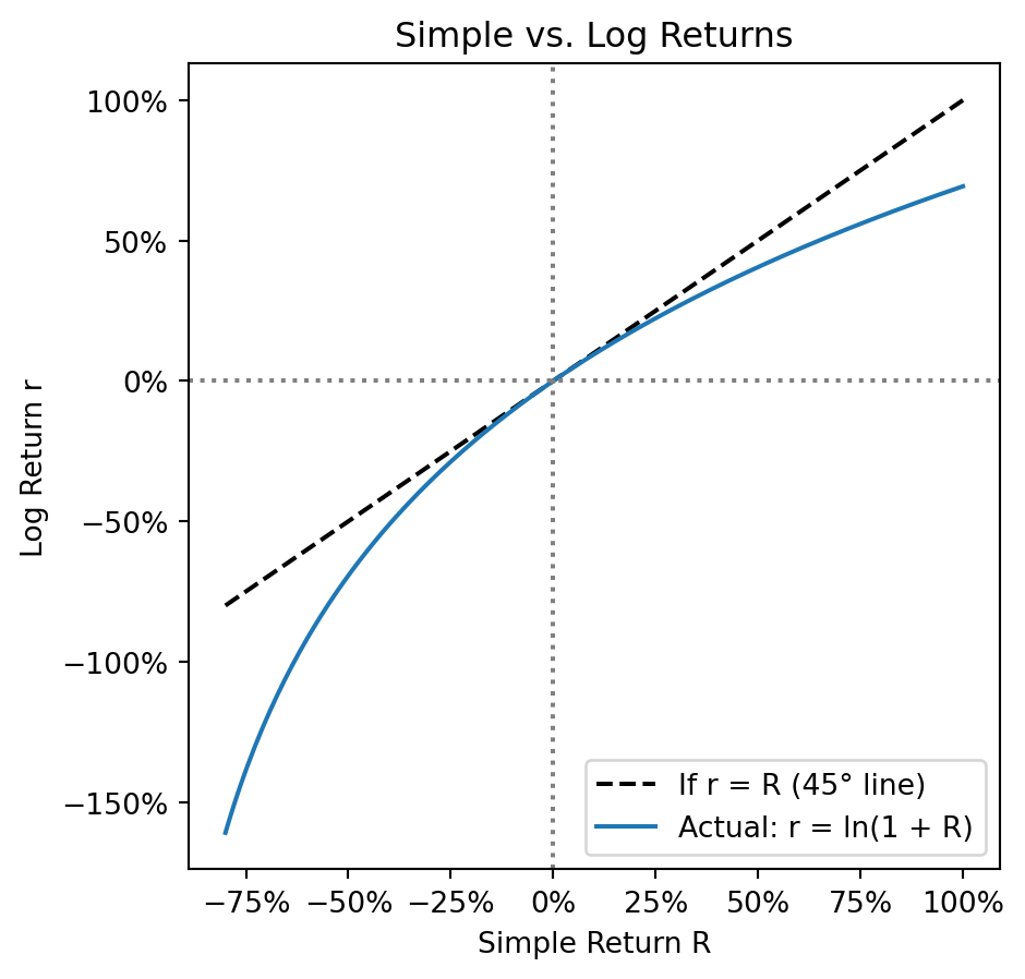
Given a simple return \(R\), what is the equivalent continuously compounded return \(r\)?

By definition, \(r\) is the rate such that continuous compounding gives the same growth:

\[e^r = 1 + R\]

Solving for \(r\):

\[r = \ln(1 + R)\]

This is why they’re called log returns—they’re literally the logarithm of gross returns.

For stocks (ignoring dividends), the gross return is \(1 + R_t = \frac{P_t}{P_{t-1}}\), so:

\[r_t = \ln\left(\frac{P_t}{P_{t-1}}\right) = \ln(P_t) - \ln(P_{t-1})\]

Log returns are just differences in log prices. This is extremely convenient for computation.

Example: If \(R = 7\%\), then \(r = \ln(1.07) \approx 6.77\%\).

Why does this help? Recall from Week 1 that \(\ln(ab) = \ln(a) + \ln(b)\).

Apply this to multi-period returns:

\[\begin{align*} r_{1 \to T} &= \ln(1 + R_{1 \to T}) = \ln\left[\prod_{t=1}^{T}(1+R_t)\right] \\ &= \ln(1+R_1) + \ln(1+R_2) + \cdots + \ln(1+R_T) \\ &= r_1 + r_2 + \cdots + r_T = \sum_{t=1}^{T} r_t \end{align*}\]

Log returns add over time. This is much easier to work with mathematically.

The annualized log return \(\bar{r}\) is the constant rate that, if earned every year, gives the same terminal wealth.

Derivation: Earning \(\bar{r}\) for \(T\) years means terminal wealth is:

\[W_T = W_0 \cdot e^{\bar{r}} \cdot e^{\bar{r}} \cdots e^{\bar{r}} = W_0 \cdot e^{T\bar{r}}\]

This must equal the actual terminal wealth \(W_0 \cdot e^{r_{1 \to T}}\):

\[W_0 \cdot e^{T\bar{r}} = W_0 \cdot e^{r_{1 \to T}}\]

Taking logs of both sides:

\[T\bar{r} = r_{1 \to T} \quad \implies \quad \bar{r} = \frac{r_{1 \to T}}{T} = \frac{1}{T}\sum_{t=1}^{T} r_t\]

The annualized log return is just the arithmetic mean! No roots, no messy exponents.

Converting Between Simple and Log Returns

Key relationships:

\[r_t = \ln(1 + R_t) \quad \Longleftrightarrow \quad R_t = e^{r_t} - 1\]

For small returns, \(r_t \approx R_t\) (because \(\ln(1+x) \approx x\) for small \(x\)). The difference grows for larger returns:

import numpy as np
import matplotlib.pyplot as plt
from matplotlib.ticker import PercentFormatter

# Simple returns from -80% to +100%
R = np.linspace(-0.8, 1.0, 200)

# Log returns: r = ln(1 + R)
r = np.log(1 + R)

fig, ax = plt.subplots(figsize=(5, 5))
ax.plot(R, R, 'k--', label='If r = R (45° line)')
ax.plot(R, r, label='Actual: r = ln(1 + R)')
ax.set_xlabel('Simple Return R')
ax.set_ylabel('Log Return r')
ax.axhline(0, linestyle=':', color='gray')
ax.axvline(0, linestyle=':', color='gray')
ax.xaxis.set_major_formatter(PercentFormatter(xmax=1))
ax.yaxis.set_major_formatter(PercentFormatter(xmax=1))
ax.legend()
ax.set_title('Simple vs. Log Returns')
plt.show()

Note the asymmetry: log returns treat gains and losses differently.

  • A 50% gain: \(r = \ln(1.5) = 40.5\%\)
  • A 50% loss: \(r = \ln(0.5) = -69.3\%\)

Why Computational Finance Prefers Log Returns

Summary of advantages:

  1. Additivity: Multi-period returns are just sums and annualizing multi-period returns is multiplicative: \[r_{1 \to T} = \sum_{t=1}^{T} r_t \qquad r_{1 \to T}^\text{annual} = \frac{1}{T} r_{1 \to T}\]

  2. Statistical convenience: Sums/scalar multiples of random variables are easier to analyze than exponentiated products

  3. No lower bound: Log returns can be any real number; simple returns are bounded below by \(-100\%\)

Simple returns are what you actually earn. Log returns are what you compute with. We’ll move between them as needed.

The Key Assumption: Log Returns Are Normal

A foundational assumption in quantitative finance:

Log returns are normally distributed.

In notation (recall from Week 1):

\[r_t \sim N(\mu, \sigma^2)\]

This says: each period’s log return is a random draw from a normal distribution with mean \(\mu\) and variance \(\sigma^2\).

We usually invest to grow our wealth, so if log returns are normally distributed, what does that imply for the distribution of prices (or wealth)?

From Log Returns to Wealth

Suppose you start with wealth \(W_0\) and invest for \(T\) years.

Your terminal wealth is the product of gross returns:

\[W_T = W_0 \cdot (1 + R_1)(1 + R_2) \cdots (1 + R_T)\]

Using the relationship \(1 + R_t = e^{r_t}\):

\[W_T = W_0 \cdot e^{r_1} \cdot e^{r_2} \cdots e^{r_T} = W_0 \cdot e^{r_1 + r_2 + \cdots + r_T}\]

Taking logs of both sides:

\[\ln\left(\frac{W_T}{W_0}\right) = r_{1 \to T} = \sum_{t=1}^{T} r_t\]

Key insight: Log wealth growth is a sum of log returns. This is why the assumption about log returns matters so much.

Why \(T\) Appears Everywhere

If each year’s log return is an independent draw from \(N(\mu, \sigma^2)\):

\[r_1, r_2, \ldots, r_T \stackrel{\text{i.i.d.}}{\sim} N(\mu, \sigma^2)\]

Then the sum of \(T\) such draws is (recall from Week 1):

\[\sum_{t=1}^{T} r_t \sim N\left(\underbrace{T \cdot \mu}_{\text{mean}}, \; \underbrace{T \cdot \sigma^2}_{\text{variance}}\right)\]

Both the mean and variance scale with \(T\):

  • Mean grows linearly: expected cumulative return is \(T\mu\)
  • Variance grows linearly: uncertainty compounds over time
  • Standard deviation grows with \(\sqrt{T}\): \(\text{SD} = \sigma\sqrt{T}\)

This is why time horizon is so important in finance.

The Distribution of Log Wealth

Combining our results:

\[\ln(W_T) = \ln(W_0) + \sum_{t=1}^{T} r_t\]

Since \(\sum_{t=1}^{T} r_t \sim N(T\mu, T\sigma^2)\), we have:

\[\ln(W_T) \sim N\left(\ln(W_0) + T\mu, \; T\sigma^2\right)\]

Log wealth is normally distributed.

But we care about wealth itself, \(W_T\), not its logarithm.

If \(\ln(W_T)\) is normal, what distribution does \(W_T\) follow?

The Log-Normal Distribution

Definition: A random variable \(X\) is log-normally distributed if \(\ln(X)\) is normally distributed.

\[\text{If } Z \sim N(m, v), \text{ then } X = e^Z \text{ is log-normal.}\]

In our case:

  • \(\ln(W_T) \sim N(\ln(W_0) + T\mu, \; T\sigma^2)\)
  • Therefore \(W_T\) is log-normally distributed

The key implication:

\[\text{Normal log returns} \implies \text{Log-normal wealth}\]

Forecasting Future Wealth

We want to forecast expected terminal wealth: \(\mathbb{E}[W_T]\)

We know:

\[W_T = W_0 \cdot e^{\sum_{t=1}^T r_t}\]

And we know \(\mathbb{E}\left[\sum r_t\right] = T\mu\).

Tempting guess: \(\mathbb{E}[W_T] = W_0 \cdot e^{T\mu}\)?

This would require:

\[\mathbb{E}\left[e^{\sum r_t}\right] \stackrel{?}{=} e^{\mathbb{E}\left[\sum r_t\right]}\]

But in general: \(\mathbb{E}[f(X)] \neq f(\mathbb{E}[X])\)

So how wrong is our guess, and in which direction?

Normal vs. Log-Normal: A Visual Comparison

import numpy as np
import matplotlib.pyplot as plt
from scipy import stats

fig, (ax1, ax2) = plt.subplots(1, 2)

# Normal distribution
x_norm = np.linspace(-3, 3, 1000)
ax1.plot(x_norm, stats.norm.pdf(x_norm))
ax1.axvline(0, linestyle='--', label='mean = median = mode')
ax1.set_xlabel('z')
ax1.set_title('Normal: Z ~ N(0,1)')
ax1.legend()

# Log-normal distribution
x_lognorm = np.linspace(0.01, 5, 1000)
ax2.plot(x_lognorm, stats.lognorm.pdf(x_lognorm, s=1, scale=1))

# Mode, median, mean for log-normal
mode = np.exp(-1)    # exp(-sigma^2)
median = 1           # exp(mu)
mean = np.exp(0.5)   # exp(mu + sigma^2/2)

ax2.axvline(mode, linestyle='--', label=f'mode = {mode:.2f}')
ax2.axvline(median, linestyle='--', label=f'median = {median:.2f}')
ax2.axvline(mean, linestyle='--', label=f'mean = {mean:.2f}')
ax2.set_xlabel('x = exp(z)')
ax2.set_title('Log-Normal: X = exp(Z)')
ax2.legend()

plt.show()

Exponentiating a symmetric distribution creates asymmetry: Mode \(<\) Median \(<\) Mean.

The key formula: If \(Z \sim N(\mu, \sigma^2)\), then the mean of \(e^Z\) (recall: mean = expected value = \(\mathbb{E}[\cdot]\)) is:

\[\mathbb{E}[e^Z] = e^{\mu + \frac{\sigma^2}{2}}\]

The variance \(\sigma^2\) appears in the expected value! This is fundamental to log-normal distributions.

Advanced: Where does this formula come from?

Recall from Week 1: for a continuous random variable, \(\mathbb{E}[g(X)] = \int g(x) \cdot f_X(x) \, dx\) where \(f_X\) is the PDF.

Here \(g(z) = e^z\) and \(f_Z(z) = \frac{1}{\sqrt{2\pi \sigma^2}} e^{-\frac{(z-\mu)^2}{2\sigma^2}}\) is the normal PDF, so:

\[\mathbb{E}[e^Z] = \int_{-\infty}^{\infty} e^z \cdot \frac{1}{\sqrt{2\pi \sigma^2}} e^{-\frac{(z-\mu)^2}{2\sigma^2}} \, dz\]

Combine the exponentials: the exponent is \(z - \frac{(z-\mu)^2}{2\sigma^2}\). Complete the square:

\[\begin{align*} z - \frac{(z-\mu)^2}{2\sigma^2} &= \frac{2\sigma^2 z - (z^2 - 2\mu z + \mu^2)}{2\sigma^2} \\ &= \frac{-z^2 + 2z(\mu + \sigma^2) - \mu^2}{2\sigma^2} \\ &= -\frac{(z - (\mu + \sigma^2))^2}{2\sigma^2} + \frac{(\mu + \sigma^2)^2 - \mu^2}{2\sigma^2} \\ &= -\frac{(z - (\mu + \sigma^2))^2}{2\sigma^2} + \mu + \frac{\sigma^2}{2} \end{align*}\]

So the integral becomes:

\[\mathbb{E}[e^Z] = e^{\mu + \frac{\sigma^2}{2}} \int_{-\infty}^{\infty} \frac{1}{\sqrt{2\pi \sigma^2}} e^{-\frac{(z - (\mu + \sigma^2))^2}{2\sigma^2}} \, dz = e^{\mu + \frac{\sigma^2}{2}} \cdot 1\]

The integral equals 1 because it’s the PDF of \(N(\mu + \sigma^2, \sigma^2)\) integrated over all \(z\).

Why Does Variance Affect the Mean?

Intuition: The exponential function \(e^z\) is convex (curves upward, second derivative positive).

By Jensen’s inequality: for a convex function \(f\) and random variable \(Z\),

\[\mathbb{E}[f(Z)] \geq f(\mathbb{E}[Z])\]

Applied to \(f(z) = e^z\):

\[e^{\mu + \frac{\sigma^2}{2}} = {\mathbb{E}[e^Z]} > e^{\mathbb{E}[Z]} = e^{\mu}\]

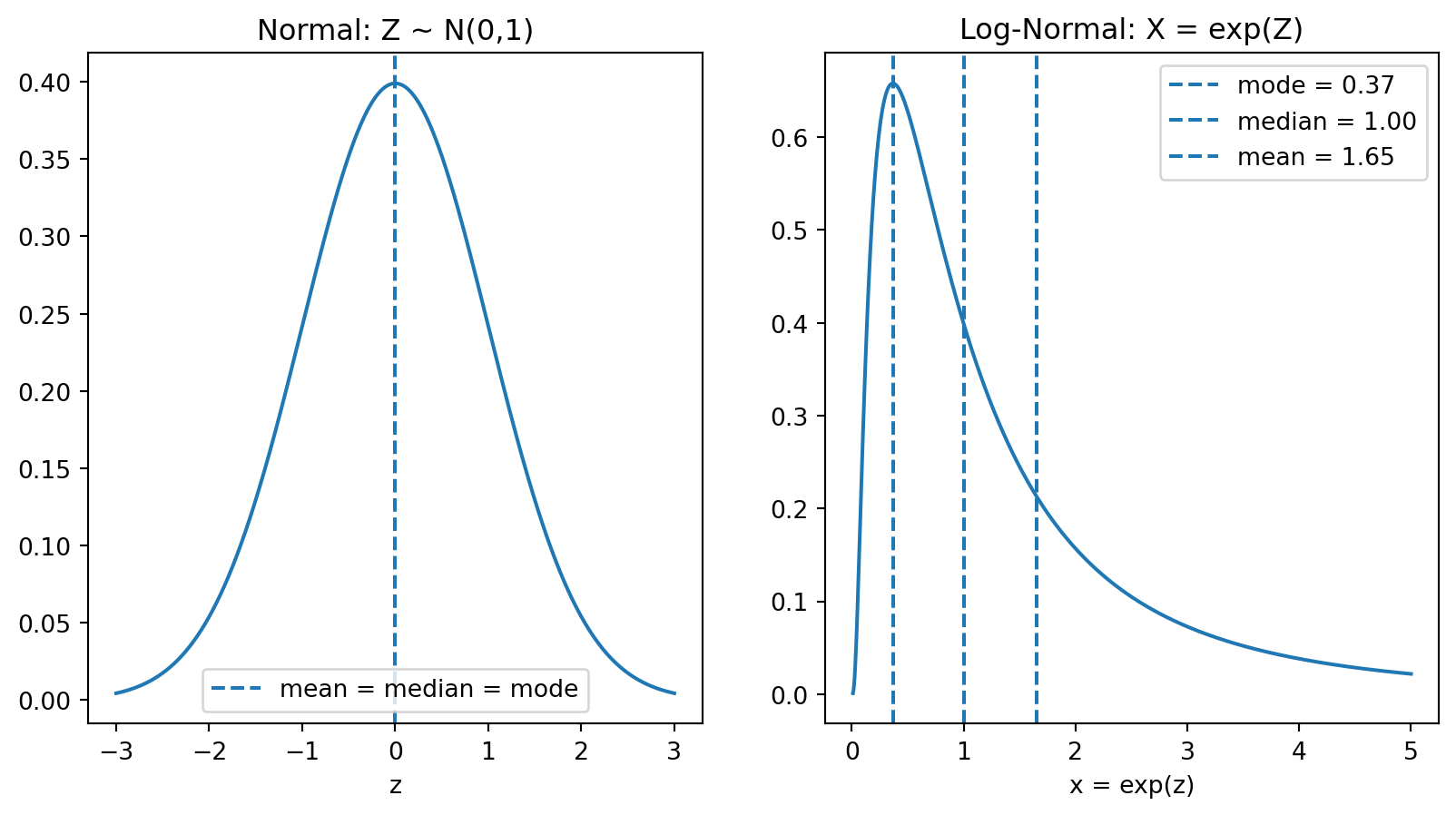
The \(\frac{\sigma^2}{2}\) term is the variance boost. The more spread out \(Z\) is (higher variance), the more the exponential “boosts” the high values relative to the low values.

Expected Wealth After \(T\) Years

Recall: our “naïve” forecast for terminal wealth (ignoring variance) was \(W_0 \cdot e^{T\mu}\).

But now we know the true expected value includes the variance boost:

\[\mathbb{E}[W_T] = W_0 \cdot e^{T\mu + \frac{T\sigma^2}{2}} = W_0 \cdot e^{T\mu} \cdot e^{\frac{T\sigma^2}{2}}\]

The factor \(e^{T\sigma^2/2}\) is the variance boost:

  • It grows with time horizon \(T\): longer investments have larger boosts
  • It grows with volatility \(\sigma^2\): riskier assets have larger boosts
  • This happens because wealth is log-normally distributed with a fat right tail: Mean \(>\) Median, and the gap widens with \(T\) and \(\sigma^2\)
  • Over long horizons, expected wealth becomes much larger than what a “typical” investor will experience

Simulating 100,000 Investors

Step 0: Estimate \(\mu\) and \(\sigma\) from real data.

Rather than using made-up numbers, let’s estimate from actual S&P 500 history.

import numpy as np
import pandas as pd
import matplotlib.pyplot as plt
from scipy import stats
import os

# Load S&P 500 data (download if not cached locally)
csv_path = 'sp500_yf.csv'
if os.path.exists(csv_path):
    sp500 = pd.read_csv(csv_path, index_col='Date', parse_dates=True)
else:
    import yfinance as yf
    sp500 = yf.download('^GSPC', start='1950-01-01', end='2025-12-31', progress=False)
    sp500.columns = sp500.columns.get_level_values(0)
    sp500.to_csv(csv_path)

# Use the last 60 years of data
T = 60  # Investment horizon (years)
end_year = sp500.index.max().year
start_year = end_year - T
sp500_recent = sp500[sp500.index.year >= start_year]

print(f"Using data from {start_year} to {end_year} ({T} years)")

# Compute daily log returns
daily_log_returns = np.log(sp500_recent['Close'] / sp500_recent['Close'].shift(1)).dropna()

# Estimate daily mu and sigma, then annualize
# (252 trading days per year)
mu_daily = daily_log_returns.mean()
sigma_daily = daily_log_returns.std()

mu = mu_daily * 252           # Annualized mean
sigma = sigma_daily * np.sqrt(252)  # Annualized volatility

print(f"\nDaily estimates:")
print(f"  μ_daily: {mu_daily:.4%}   σ_daily: {sigma_daily:.4%}")
print(f"\nAnnualized (×252 for μ, ×√252 for σ):")
print(f"  μ (mean annual log return): {mu:.2%}")
print(f"  σ (annual volatility):      {sigma:.2%}")
Using data from 1965 to 2025 (60 years)

Daily estimates:
  μ_daily: 0.0286%   σ_daily: 1.0555%

Annualized (×252 for μ, ×√252 for σ):
  μ (mean annual log return): 7.22%
  σ (annual volatility):      16.76%

Now we can compute forecasts:

  • Median (naïve forecast): \(e^{T\mu}\) — what you get if returns equal their mean every year
  • Mean (true expected value): \(e^{T\mu + T\sigma^2/2}\) — includes the variance boost
W_0 = 1  # Starting wealth = $1

median_wealth = W_0 * np.exp(T * mu)
mean_wealth = W_0 * np.exp(T * mu + T * sigma**2 / 2)

print(f"Starting wealth: ${W_0}")
print(f"Horizon: {T} years")
print(f"\nMedian terminal wealth (naïve): ${median_wealth:,.0f}")
print(f"Mean terminal wealth (true E[W]):  ${mean_wealth:,.0f}")
print(f"\nThe mean is {mean_wealth/median_wealth:.1f}× higher than the median!")
Starting wealth: $1
Horizon: 60 years

Median terminal wealth (naïve): $76
Mean terminal wealth (true E[W]):  $177

The mean is 2.3× higher than the median!

The mean is pulled up by a small number of extremely lucky outcomes—most investors will earn less than the expected value. Let’s simulate this.

np.random.seed(42)
n_investors = 100000

# Step 1: Draw 60 years of log returns for each investor
# Each row = one investor, each column = one year
returns = np.random.normal(mu, sigma, (n_investors, T))

print(f"Shape: {returns.shape} (100,000 investors × {T} years)")
print(f"First investor's first 5 years: {returns[0, :5].round(3)}")
Shape: (100000, 60) (100,000 investors × 60 years)
First investor's first 5 years: [0.155 0.049 0.181 0.327 0.033]

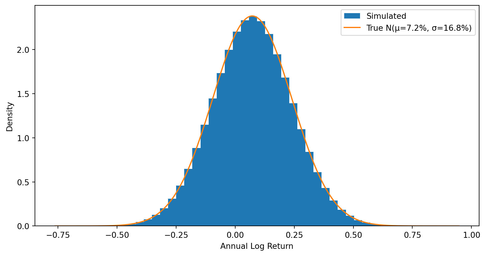
Each investor gets 60 independent draws from \(N(\mu, \sigma^2)\).

Step 1: Individual annual returns are normally distributed (symmetric).

# The distribution of individual annual returns
all_returns = returns.flatten()

plt.hist(all_returns, bins=50, density=True, label='Simulated')

# Overlay the true normal distribution
x = np.linspace(all_returns.min(), all_returns.max(), 200)
plt.plot(x, stats.norm.pdf(x, mu, sigma), label=f'True N(μ={mu:.1%}, σ={sigma:.1%})')

plt.xlabel('Annual Log Return')
plt.ylabel('Density')
plt.legend()
plt.show()

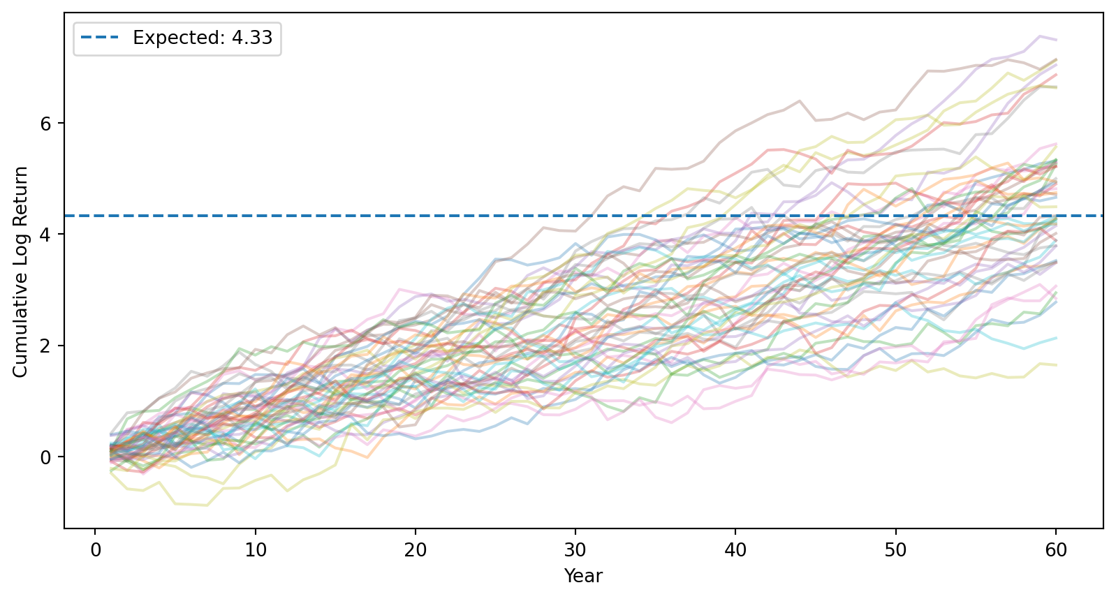
Step 2: Log returns accumulate over time (still symmetric).

# Cumulative log returns (running sum over time)
cumulative_log_returns = np.cumsum(returns, axis=1)

# Plot sample paths for a few investors
for i in range(50):
    plt.plot(range(1, T+1), cumulative_log_returns[i], alpha=0.3)

plt.axhline(mu * T, linestyle='--', label=f'Expected: {mu*T:.2f}')
plt.xlabel('Year')
plt.ylabel('Cumulative Log Return')
plt.legend()
plt.show()

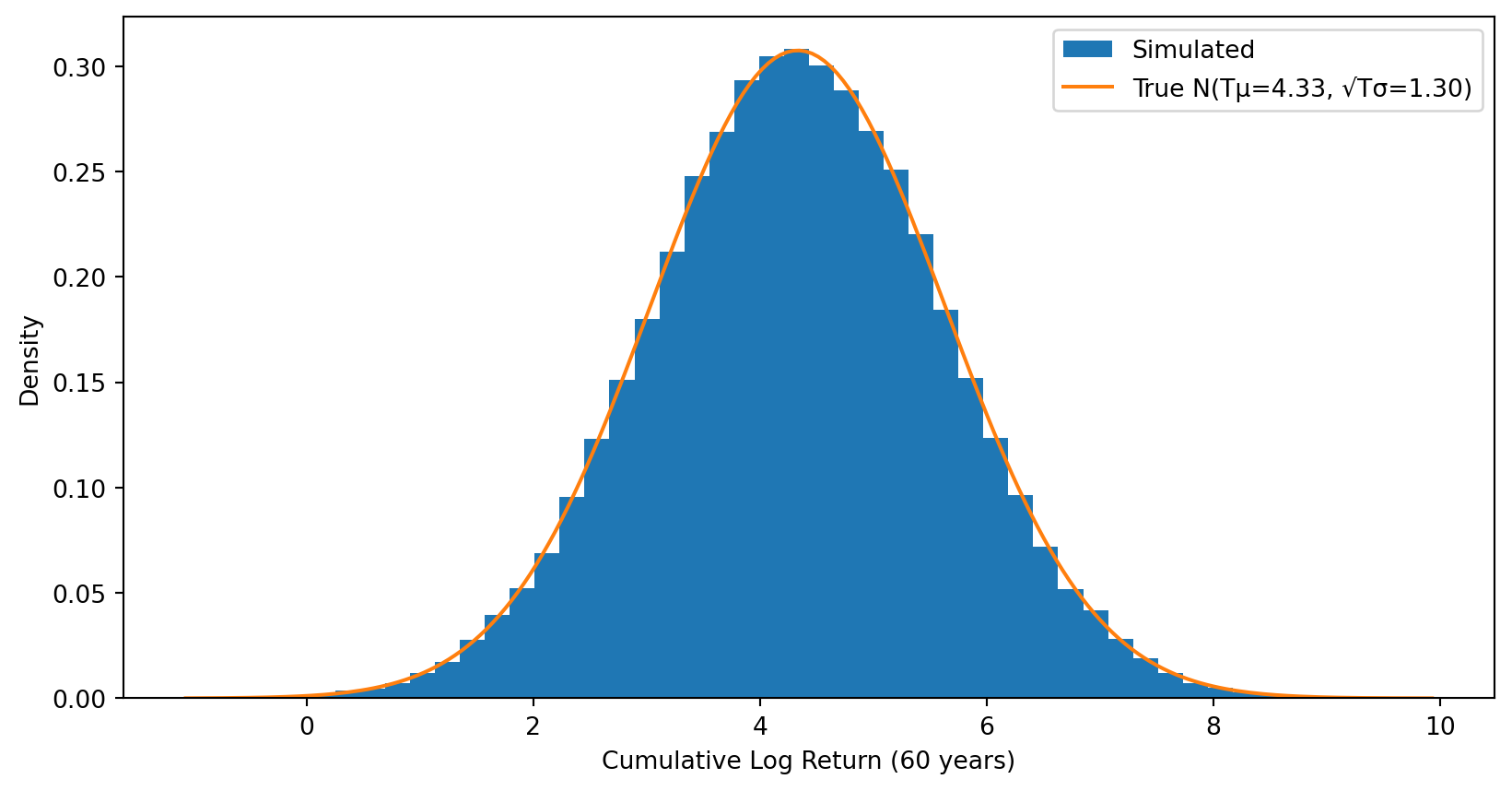
After \(T\) years, cumulative log return \(\sim N(T\mu, T\sigma^2)\) — still symmetric.

# Distribution of terminal cumulative log returns
terminal_log_returns = cumulative_log_returns[:, -1]

plt.hist(terminal_log_returns, bins=50, density=True, label='Simulated')

# Overlay the true normal distribution: N(T*mu, T*sigma^2)
x = np.linspace(terminal_log_returns.min(), terminal_log_returns.max(), 200)
plt.plot(x, stats.norm.pdf(x, mu*T, sigma*np.sqrt(T)),
         label=f'True N(Tμ={mu*T:.2f}, √Tσ={sigma*np.sqrt(T):.2f})')

plt.xlabel(f'Cumulative Log Return ({T} years)')
plt.ylabel('Density')
plt.legend()
plt.show()

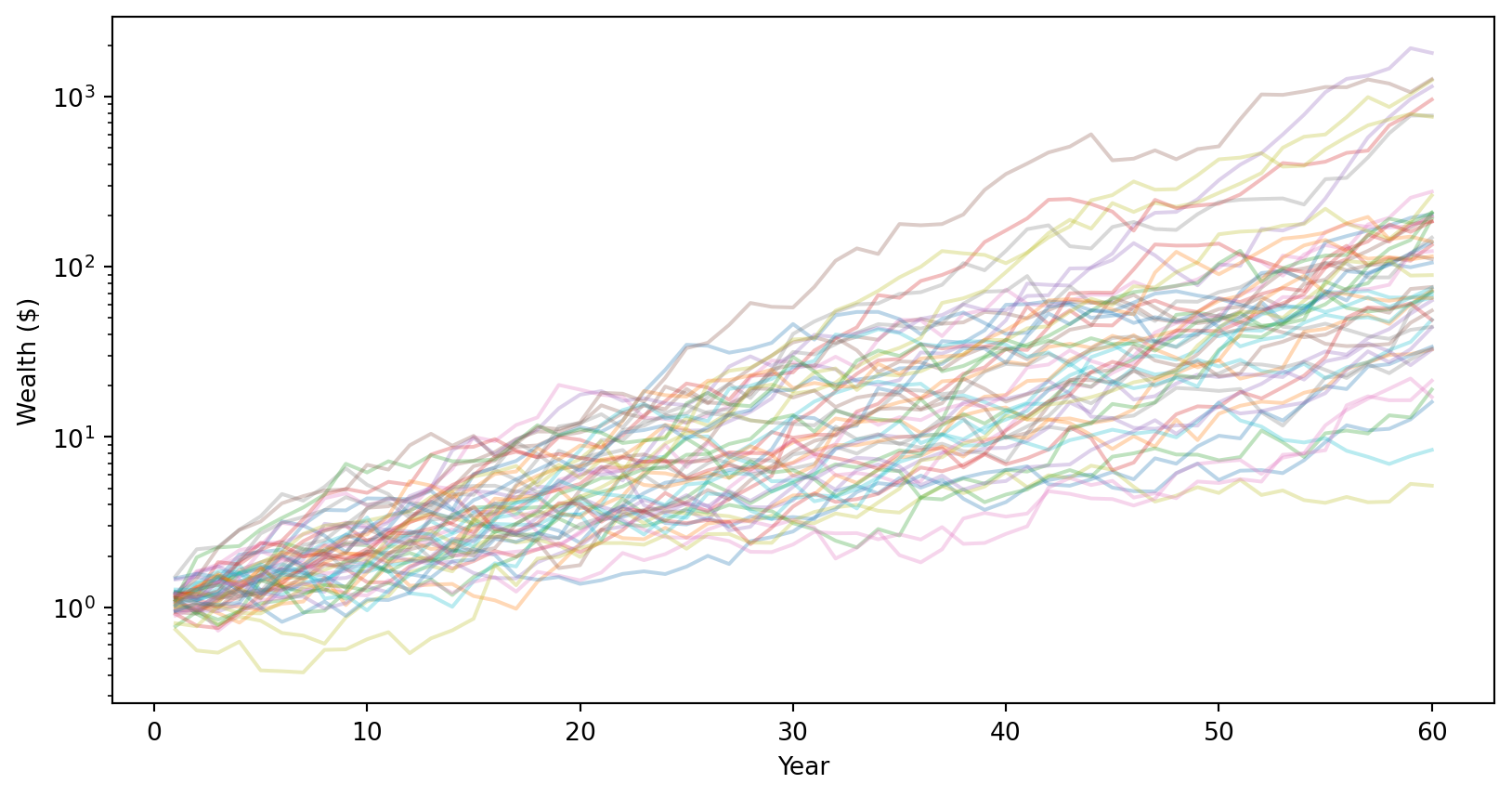
Step 3: Exponentiate to get wealth (now asymmetric!).

# Convert to wealth by exponentiating: W_T = W_0 * exp(cumulative log return)
wealth_paths = W_0 * np.exp(cumulative_log_returns)

# Plot sample paths
for i in range(50):
    plt.plot(range(1, T+1), wealth_paths[i], alpha=0.3)

plt.xlabel('Year')
plt.ylabel('Wealth ($)')
plt.yscale('log')  # Log scale to see all paths
plt.show()

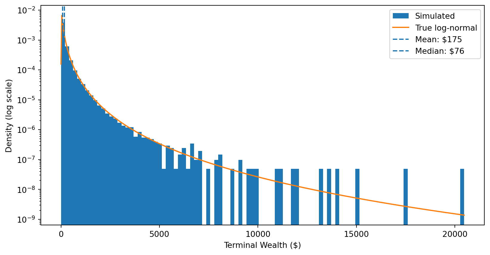
Step 4: Terminal wealth is log-normally distributed.

# Final wealth after T years
terminal_wealth = wealth_paths[:, -1]

plt.hist(terminal_wealth, bins=100, density=True, label='Simulated')

# Overlay the true log-normal distribution
# If ln(W) ~ N(m, v), then W is log-normal with scale=exp(m) and s=sqrt(v)
x = np.linspace(terminal_wealth.min(), terminal_wealth.max(), 500)
plt.plot(x, stats.lognorm.pdf(x, s=sigma*np.sqrt(T), scale=np.exp(mu*T)), label='True log-normal')

plt.axvline(np.mean(terminal_wealth), linestyle='--', label=f'Mean: ${np.mean(terminal_wealth):.0f}')
plt.axvline(np.median(terminal_wealth), linestyle='--', label=f'Median: ${np.median(terminal_wealth):.0f}')
plt.xlabel('Terminal Wealth ($)')
plt.ylabel('Density (log scale)')
# plt.xscale('log')
plt.yscale('log')
plt.legend()
plt.show()

print(f"{100*np.mean(terminal_wealth < np.mean(terminal_wealth)):.0f}% of investors earn less than the mean!")

74% of investors earn less than the mean!

The punchline: Most investors earn less than the expected value!

The Punchline: Expected Value Is Biased Upward

Summary of Part I:

  1. Log returns assumed normal \(\implies\) wealth is log-normal
  2. The expected value of a log-normal includes a variance boost: \(e^{T\sigma^2/2}\)
  3. This boost grows with time horizon \(T\) and volatility \(\sigma^2\)
  4. As a result: Mean \(>\) Median \(>\) Mode for terminal wealth

The implication:

If you use expected wealth to plan for retirement (or advise clients), you will systematically overestimate what most people will actually experience.

Next: How do we adjust for this bias? And where does the uncertainty come from?

Part II: Estimation Risk

From Known to Unknown Parameters

In Part I, we treated \(\mu\) and \(\sigma^2\) as known parameters.

Reality: We don’t know the true expected return \(\mu\). We must estimate it from historical data.

This introduces estimation risk—additional uncertainty because our parameters are estimates, not truth.

Key question: If we plug our estimate \(\hat{\mu}\) into the wealth formula, do we get an unbiased forecast of expected wealth?

Spoiler: No. There’s an additional source of upward bias beyond what we saw in Part I.

What Is an Unbiased Estimator?

Definition: An estimator \(\hat{\theta}\) is unbiased if its expected value equals the true parameter:

\[\mathbb{E}[\hat{\theta}] = \theta\]

Example: The sample mean \(\bar{r} = \frac{1}{N}\sum_{i=1}^{N} r_i\) is an unbiased estimator of \(\mu\).

Why should we care?

  • Unbiased estimators are correct on average over repeated sampling
  • They avoid systematic over- or under-prediction
  • In finance: unbiased forecasts prevent consistently overoptimistic (or pessimistic) investment expectations

Caution: An unbiased estimator of \(\mu\) does not automatically give an unbiased estimator of functions of \(\mu\) (like \(e^{T\mu}\)).

Estimating the Mean Return

Setup: We have \(N\) historical observations of log returns: \(r_1, r_2, \ldots, r_N\). (For now, assume we know the true volatility \(\sigma\).)

We estimate the true mean \(\mu\) using the sample mean:

\[\hat{\mu} = \frac{1}{N} \sum_{i=1}^{N} r_i\]

Properties of \(\hat{\mu}\):

  • Unbiased: \(\mathbb{E}[\hat{\mu}] = \mu\)
  • Standard error: \(\text{SE}(\hat{\mu}) = \frac{\sigma}{\sqrt{N}}\)
  • Distribution: \(\hat{\mu} \sim N\left(\mu, \frac{\sigma^2}{N}\right)\)

The standard error \(\frac{\sigma}{\sqrt{N}}\) tells us how uncertain we are about \(\mu\). More data (larger \(N\)) means less uncertainty.

Standard Error: How Precise Is Our Estimate?

The standard error of \(\hat{\mu}\) is the standard deviation of our estimator:

\[SE(\hat{\mu}) = \frac{\sigma}{\sqrt{N}}\]

Example: With \(\sigma = 20\%\) annual volatility:

Years of data (\(N\)) Standard error
25 years \(\frac{0.20}{\sqrt{25}} = 4\%\)
50 years \(\frac{0.20}{\sqrt{50}} = 2.8\%\)
100 years \(\frac{0.20}{\sqrt{100}} = 2\%\)

Even with 100 years of data, our estimate of \(\mu\) is only accurate to about \(\pm 2\%\).

If \(\mu \approx 8\%\), a 2% standard error means we’re quite uncertain about the true value!

The Estimated Wealth Forecast

Suppose we want to forecast expected wealth over \(T\) periods using our estimate \(\hat{\mu}\).

From Part I, we know true expected wealth is \(\mathbb{E}[W_T] = W_0 \exp\left(T\mu + \frac{T\sigma^2}{2}\right)\).

Natural approach: Plug in our estimate:

\[\widehat{W}_T = W_0 \cdot \exp\left(T\hat{\mu} + \frac{T\sigma^2}{2}\right)\]

(For simplicity, assume \(\sigma^2\) is known.)

Question: Is \(\widehat{W}_T\) an unbiased estimator of \(\mathbb{E}[W_T]\)?

In other words: Does \(\mathbb{E}[\widehat{W}_T] = \mathbb{E}[W_T]\)?

The Bias in Estimated Wealth

Answer: No! \(\widehat{W}_T\) is upward biased.

Why? Since \(\hat{\mu} \sim N\left(\mu, \frac{\sigma^2}{N}\right)\), we have \(T\hat{\mu} \sim N\left(T\mu, \frac{T^2\sigma^2}{N}\right)\).

Now \(\exp(T\hat{\mu})\) is log-normal! Using our formula from Part I:

\[\mathbb{E}[\exp(T\hat{\mu})] = \exp\left(T\mu + \frac{T^2\sigma^2}{2N}\right)\]

Putting it together:

\[\begin{align*} \mathbb{E}[\widehat{W}_T] &= W_0 \cdot \mathbb{E}[\exp(T\hat{\mu})] \cdot \exp\left(\frac{T\sigma^2}{2}\right) \\ &= \underbrace{W_0 \cdot \exp\left(T\mu + \frac{T\sigma^2}{2}\right)}_{\mathbb{E}[W_T]} \cdot \underbrace{\exp\left(\frac{T^2\sigma^2}{2N}\right)}_{\text{Bias Factor}} \end{align*}\]

Key result:

\[\boxed{\mathbb{E}[\widehat{W}_T] = \mathbb{E}[W_T] \cdot \exp\left(\frac{T^2\sigma^2}{2N}\right)}\]

The bias factor is always \(> 1\), so \(\widehat{W}_T\) systematically overestimates expected wealth.

Intuition: Why Does Estimation Error Create Upward Bias?

The same Jensen’s inequality logic from Part I applies here.

  • Our estimate \(\hat{\mu}\) is sometimes too high, sometimes too low
  • When \(\hat{\mu}\) is too high, \(\exp(T\hat{\mu})\) overshoots by a lot
  • When \(\hat{\mu}\) is too low, \(\exp(T\hat{\mu})\) undershoots by less
  • On average, the overshoots win—the mean is pulled up

The exponential function is convex: it amplifies high values more than it dampens low values.

This is exactly the same mechanism that made \(\mathbb{E}[W_T] > \text{Median}[W_T]\) in Part I.

Bottom line: Any uncertainty that enters the exponent inflates the expected value.

Correcting the Bias: An Unbiased Estimator

To get an unbiased estimator of \(\mathbb{E}[W_T]\), we subtract the bias term:

\[\boxed{\widehat{W}_T^{\text{unbiased}} = W_0 \cdot \exp\left(T\hat{\mu} + \frac{T\sigma^2}{2} - \frac{T^2\sigma^2}{2N}\right)}\]

The correction term \(\frac{T^2\sigma^2}{2N}\) removes the upward bias caused by estimation risk.

Reference: This adjustment is derived in Jacquier, Kane, and Marcus (2003), “Geometric or Arithmetic Mean: A Reconsideration,” Financial Analysts Journal.

Intuition: We’re subtracting out the “extra variance” that comes from not knowing \(\mu\) perfectly.

Two Sources of Uncertainty

Our wealth forecast faces two distinct sources of uncertainty:

  1. Return risk: Future returns are random
    • Variance contribution to \(\ln(W_T)\): \(T\sigma^2\)
    • Grows linearly with horizon \(T\)
  2. Estimation risk: We don’t know \(\mu\) exactly
    • Variance contribution to forecast: \(\frac{T^2\sigma^2}{N}\)
    • Grows with \(T^2\)—much faster!

Total variance in log wealth forecast:

\[\text{Var}[\ln(\widehat{W}_T)] = T\sigma^2 + \frac{T^2\sigma^2}{N}\]

Summary of Part II

Key takeaways:

  1. While \(\hat{\mu}\) is an unbiased estimator of \(\mu\), the wealth forecast \(\widehat{W}_T\) is not an unbiased estimator of \(\mathbb{E}[W_T]\)

  2. The bias factor is \(\exp\left(\frac{T^2\sigma^2}{2N}\right)\)—it grows with \(T^2\)

  3. We can correct for this bias by subtracting \(\frac{T^2\sigma^2}{2N}\) from the exponent

  4. Estimation risk grows faster than return risk as horizon increases

Practical implication: Be skeptical of long-horizon wealth projections. They compound two sources of upward bias: the log-normal effect (Part I) and estimation error (Part II).

Part III: Testing the Normality Assumption

Are Returns Actually Normal?

Everything so far relied on one key assumption:

\[r_t \sim N(\mu, \sigma^2)\]

Is this actually true?

To investigate, we need tools to measure how a distribution deviates from normality:

  • Skewness: Is the distribution symmetric?
  • Kurtosis: How heavy are the tails?

For a normal distribution: skewness \(= 0\) and excess kurtosis \(= 0\).

Let’s see what the data say.

Skewness and Kurtosis

Skewness measures asymmetry:

\[\gamma_1 = \frac{\mathbb{E}[(R - \mu)^3]}{\sigma^3}\]

  • \(\gamma_1 = 0\): Symmetric (normal)
  • \(\gamma_1 < 0\): Left tail is longer (negative skew)—large losses more common than large gains

Kurtosis measures tail heaviness (we use excess kurtosis, relative to normal):

\[\gamma_2 = \frac{\mathbb{E}[(R - \mu)^4]}{\sigma^4} - 3\]

  • \(\gamma_2 = 0\): Normal tails
  • \(\gamma_2 > 0\): “Fat tails”—extreme events more likely than normal predicts

In finance: Stock returns typically exhibit slight negative skewness and high positive kurtosis.

Empirical Evidence: S&P 500 Returns

# Compute daily log returns (sp500 already loaded above)
sp500['log_return'] = np.log(sp500['Close'] / sp500['Close'].shift(1))
daily_returns = sp500['log_return'].dropna()

print(f"Data: {daily_returns.index.min().strftime('%Y-%m-%d')} to {daily_returns.index.max().strftime('%Y-%m-%d')}")
print(f"Observations: {len(daily_returns):,} daily returns")

# Summary statistics
skew = stats.skew(daily_returns)
kurt = stats.kurtosis(daily_returns)  # excess kurtosis

print(f"\nSkewness: {skew:.3f}  (normal = 0)")
print(f"Excess kurtosis: {kurt:.1f}  (normal = 0)")

# Test statistics (under normality, these are approx standard normal)
n_obs = len(daily_returns)
z_skew = skew / np.sqrt(6/n_obs)
z_kurt = kurt / np.sqrt(24/n_obs)

print(f"\nTest statistics (reject normality if |z| > 1.96):")
print(f"  z_skewness = {z_skew:.1f}")
print(f"  z_kurtosis = {z_kurt:.1f}")
Data: 1950-01-04 to 2025-12-19
Observations: 19,113 daily returns

Skewness: -0.953  (normal = 0)
Excess kurtosis: 25.3  (normal = 0)

Test statistics (reject normality if |z| > 1.96):
  z_skewness = -53.8
  z_kurtosis = 713.2

Result: Overwhelming evidence against normality. Kurtosis \(\approx 25\) means extreme events are far more common than normal predicts.

Fat Tails: Extreme Events Happen More Than Expected

# Standardize daily returns (already computed above)
daily_mu = daily_returns.mean()
daily_sigma = daily_returns.std()
standardized = (daily_returns - daily_mu) / daily_sigma

# Count extreme events
print("Extreme events (beyond k standard deviations):\n")
print(f"{'k-sigma':<10} {'Actual':<10} {'Normal predicts':<18} {'Ratio':<10}")
print("-" * 50)
for k in [3, 4, 5, 6]:
    actual = (abs(standardized) > k).sum()
    expected = len(daily_returns) * 2 * stats.norm.sf(k)
    ratio = actual / expected if expected > 0 else np.inf
    # Use scientific notation for very small expected values
    exp_str = f"{expected:.1f}" if expected >= 0.1 else f"{expected:.1e}"
    print(f"{k}-sigma    {actual:<10} {exp_str:<18} {ratio:,.0f}x")

# Worst day
worst_day = daily_returns.idxmin()
worst_return = daily_returns.min()
worst_sigma = (worst_return - daily_mu) / daily_sigma
print(f"\nWorst day: {worst_day.strftime('%B %d, %Y')} (Black Monday)")
print(f"Return: {worst_return:.1%}")
print(f"That's {abs(worst_sigma):.0f} standard deviations from the mean!")
Extreme events (beyond k standard deviations):

k-sigma    Actual     Normal predicts    Ratio     
--------------------------------------------------
3-sigma    272        51.6               5x
4-sigma    107        1.2                88x
5-sigma    53         1.1e-02            4,837x
6-sigma    35         3.8e-05            928,055x

Worst day: October 19, 1987 (Black Monday)
Return: -22.9%
That's 23 standard deviations from the mean!

Key insight: The normal distribution dangerously underestimates tail risk. 4-sigma events happen ~90× more often than normality predicts.

What This Means for Practice

The normality assumption is an approximation.

  • Works reasonably well for “typical” days
  • Fails badly for extreme events (crashes, rallies)

Implications:

  • Risk management: VaR and other risk measures based on normality underestimate tail risk
  • Option pricing: Black-Scholes assumes normality; real option prices reflect fat tails
  • Portfolio optimization: Mean-variance optimization ignores higher moments

For this course: We’ll continue using normal-based methods because they’re tractable and widely used—but always remember the limitation.

Part IV: Why Prediction Is Hard

Can We Predict Returns?

Autocorrelation: Does yesterday’s return predict today’s?

If returns were predictable from their own past, we could profit from it.

Empirical finding: Autocorrelations in stock returns are tiny (typically \(|\rho| < 0.05\)).

  • Statistically significant with enough data? Sometimes.
  • Economically significant after transaction costs? Rarely.

Using other predictors: What about dividend yield, P/E ratio, interest rates?

Researchers have tested hundreds of variables. The sobering result:

Goyal and Welch (2008)

Most variables that predict returns in-sample fail to predict out-of-sample. The simple historical average is hard to beat.

“A Comprehensive Look at the Empirical Performance of Equity Premium Prediction,” Review of Financial Studies

In-Sample vs. Out-of-Sample: A Preview

In-sample: How well does the model fit the data used to estimate it?

Out-of-sample: How well does the model predict new data it hasn’t seen?

The problem: In-sample performance is overly optimistic.

  • Coefficients are “tuned” to fit the specific noise in the estimation sample
  • This is called overfitting—the model fits noise, not signal
  • Out-of-sample, the noise is different, so the fit degrades

This is why ML exists. Much of this course is about techniques to avoid overfitting and improve out-of-sample performance:

  • Cross-validation
  • Regularization
  • Ensemble methods

We’ll return to IS/OOS evaluation in depth when we cover regression (Week 5).

Summary and Looking Ahead

Today’s Key Results

Part I: From Returns to Wealth

  • Log returns assumed normal \(\implies\) wealth is log-normal
  • Expected wealth includes a variance boost: \(\mathbb{E}[W_T] = W_0 e^{T\mu + T\sigma^2/2}\)
  • Mean \(>\) Median: most investors earn less than the expected value

Part II: Estimation Risk

  • We estimate \(\mu\) with error; this adds additional upward bias
  • Bias factor \(e^{T^2\sigma^2/2N}\) grows with horizon squared
  • Long-horizon wealth projections are doubly biased

Part III: The Normality Assumption Is Approximate

  • Returns have fat tails (excess kurtosis \(\approx 25\))
  • Extreme events happen far more often than normal predicts
  • Black Monday (1987): a 23-sigma event under normality

Part IV: Prediction Is Hard

  • Autocorrelations are tiny; most predictors fail out-of-sample
  • Overfitting is the enemy; out-of-sample testing is essential

What’s Next

Next week: Introduction to Machine Learning

  • What is ML? Traditional programming vs. learning from data
  • Types of learning: supervised, unsupervised, reinforcement
  • The ML formalism: models, loss functions, algorithms
  • Regression vs. classification

The rest of the course:

  • Clustering, regression, classification
  • Regularization and cross-validation
  • Ensemble methods, neural networks, text analysis

Today’s foundation carries through: We’re always estimating something from noisy data, always at risk of overfitting, always needing to check out-of-sample.