In traditional programming, you write explicit rules for the computer to follow: “if the price drops 10%, sell.” You specify the logic.
Machine learning is different. Instead of writing rules, you show the computer examples and let it discover patterns from the statistical properties of the data. The computer learns what predicts what.
Finance generates enormous amounts of data: prices, returns, fundamentals, news, filings, transactions. Machine learning gives us tools to extract information from all of it.
Think of ML methods as tools in a toolbox. Just as an experienced contractor knows which tool is right for each job—hammer for nails, wrench for bolts—you’ll learn which ML method is right for each problem:
Regression: Predicting a continuous value (next month’s return)
Classification: Assigning to categories (default vs. no default)
Text analysis: Extracting information from documents (earnings calls, news)
Why Machine Learning in Finance?
Traditional finance models are elegant but limited:
CAPM says expected returns depend on one factor (market beta)
Fama-French adds size and value
But there are hundreds of potential predictors…
The efficient frontier depends on only risk-return tradeoffs and has few conditions
But real investors may have other constraints
Do we have good estimates of risk and return?
Machine learning lets us:
Handle many variables at once without manual selection
Capture nonlinear relationships
Let the data tell us what matters
The catch: finance is noisy. Patterns that look predictive often aren’t. A major theme of this course is learning to distinguish real signal from noise.
Course Structure
Week
Topic
1
Math Bootcamp (today)
2
Financial Data
3
Introduction to Machine Learning
4
Clustering
5
Regression
6
ML & Portfolio Theory
7
Linear Classification
8
Nonlinear Classification
9
Ensemble Methods
10
Neural Networks
11
Text & NLP
12
Review
Week 1 builds the mathematical foundation. Everything else builds on it.
Today’s Goal: Increase your fluency looking at mathematical expressions, recall properties of math that drive intuition. We will NOT need to solve math problems by hand or complete any proofs.
About Me
Kevin Mott
BS in Mathematics (Northeastern University, Boston, USA)
PhD in Financial Economics (Carnegie Mellon University, Pittsburgh, USA)
Research: Deep learning methods for macro-finance problems
I study how neural networks can solve complex economic models
In macroeconomics, we can’t run experiments. How to analyze policy? Simulating the macroeconomy with neural networks.
In finance, pricing interest rate derivatives has always been hard. But neural networks can solve the pricing equations efficiently.
Symmetry: A +50% log return followed by -50% gets you back to start
Normality: Log returns are closer to normally distributed
Common math functions like \(e^x\) and \(\ln(x)\) are in the numpy library, which by convention we import as np:
import numpy as np# Computing log returns from pricesprices = np.array([100, 105, 102, 108, 110])log_returns = np.log(prices[1:]) - np.log(prices[:-1])print(f"Prices: {prices}")print(f"Log returns: {log_returns}")print(f"Sum of log returns: {log_returns.sum():.4f}")print(f"ln(final/initial): {np.log(prices[-1]/prices[0]):.4f}") # Same!
Prices: [100 105 102 108 110]
Log returns: [ 0.04879016 -0.02898754  0.05715841  0.01834914]
Sum of log returns: 0.0953
ln(final/initial): 0.0953
Part I: Statistics
What Is a Random Variable?
A random variable is a quantity whose value is determined by chance.
Examples:
Tomorrow’s S&P 500 return
The outcome of rolling a die
Whether a borrower defaults on a loan
We don’t know the exact value in advance. So how can we make informed guesses about future stock returns, or assess credit risk, or predict anything at all?
Notation: We typically use capital letters like \(X\), \(Y\), \(R\) for random variables. When we write \(X = 3\), we mean “the random variable \(X\) takes the value 3.”
From Data to Distributions
We can’t predict the exact value of a random variable. But we often have historical data—past realizations of the same random process.
By looking at many past realizations, we can see patterns: some outcomes happen frequently, others are rare. This pattern of “how likely is each outcome?” is called a distribution.
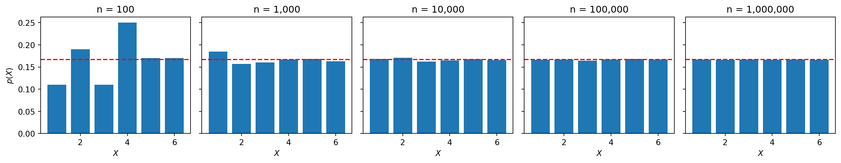
Let \(X\) be the random variable representing which side of the die is revealed.
With only 100 rolls, the pattern is noisy. With a million rolls, it’s nearly perfect—each value of \(X\) appears almost exactly 1/6 of the time (red dashed line). More data gives us a clearer picture of the true distribution.
This is a uniform distribution: each outcome equally likely.
When we write \(X \sim \text{Distribution}\), we’re saying: “the random variable \(X\) follows this pattern.”
Once we know (or estimate) a distribution, we can compute useful summary quantities:
The expected value\(\mathbb{E}[X]\) — the average outcome if we repeated the process many times
The variance\(\text{Var}(X)\) — how spread out the outcomes are around the mean
The probability of specific events — how likely is a 10% loss? A default?
These are the building blocks of statistical estimation and prediction.
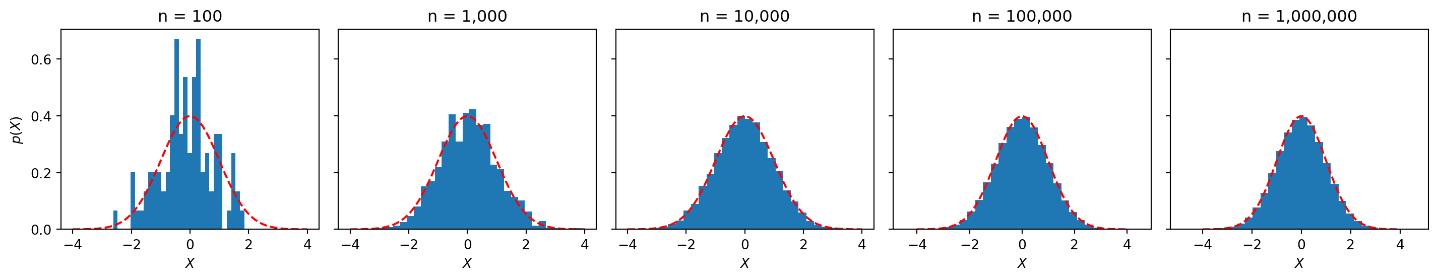
The Normal Distribution
The normal distribution (or Gaussian) is the “bell curve.” Most values cluster near the center, with extreme values increasingly rare.
We write: \(X \sim \mathcal{N}(\mu, \sigma^2)\)
\(\mu\) (mu) = the center (mean)
\(\sigma\) (sigma) = how spread out it is (standard deviation)
Same pattern: with more data, the histogram converges to the true bell curve (red dashed line).
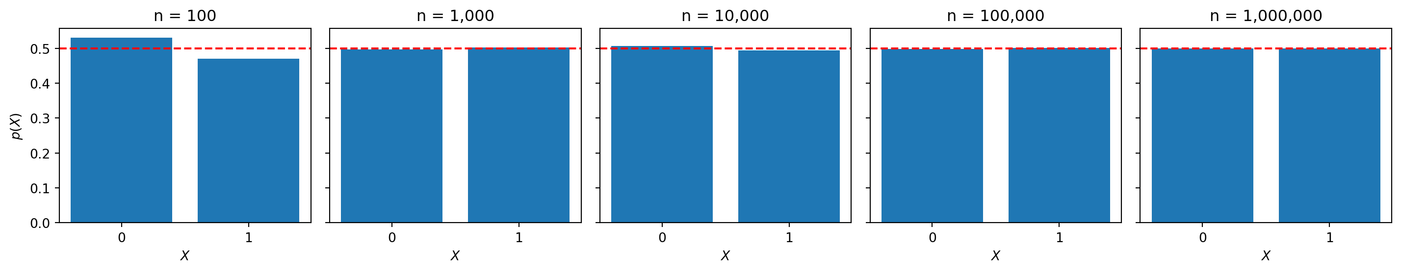
The Bernoulli Distribution
The Bernoulli distribution models yes/no outcomes: something happens (1) or doesn’t (0).
We write: \(X \sim \text{Bernoulli}(p)\)
\(p\) = probability of success (getting a 1)
\(1 - p\) = probability of failure (getting a 0)
Finance examples: Does a borrower default? Does a stock beat the market? Is a transaction fraudulent?
Let \(X = 1\) if a coin flip is heads, \(X = 0\) if tails, with \(p = 0.5\). Same pattern as before: more flips = better estimate of the true probability.
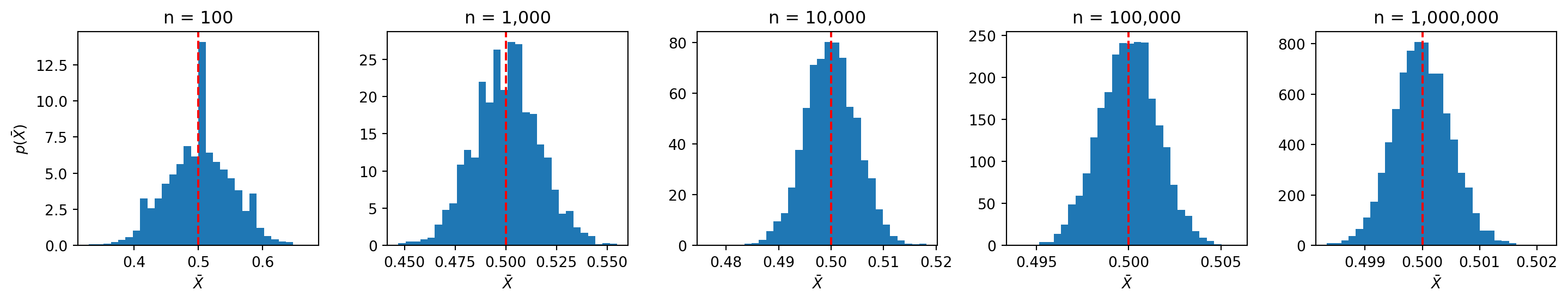
Here’s something remarkable. Suppose we run many experiments, each with \(n\) coin flips, and compute the sample mean \(\bar{X} = \frac{1}{n}\sum_{i=1}^n X_i\) in each experiment. What does the distribution of \(\bar{X}\) look like?
np.random.seed(42)p =0.5n_experiments =5000sample_sizes = [100, 1000, 10000, 100000, 1000000]fig, axes = plt.subplots(1, 5, figsize=(15, 3))for ax, n inzip(axes, sample_sizes):# Run 5000 experiments, each with n flips sample_means = np.random.binomial(n, p, size=n_experiments) / n ax.hist(sample_means, bins=30, density=True) ax.axvline(p, color='red', linestyle='--') # True mean ax.set_title(f'n = {n:,}') ax.set_xlabel('$\\bar{X}$')axes[0].set_ylabel('$p(\\bar{X})$')plt.tight_layout()plt.show()
Two things happen as \(n\) increases:
The estimates get better — the distribution of \(\bar{X}\) concentrates around the true mean. This is the law of large numbers.
The distribution becomes normal — no matter what the underlying distribution looks like (here: just 0s and 1s), the distribution of sample means becomes a bell curve. This is the central limit theorem.
In fact, the CLT tells us exactly how the sample mean is distributed:
The spread of our estimates shrinks like \(\sigma / \sqrt{n}\). To cut your estimation error in half, you need four times as much data.
Discrete vs. Continuous Distributions
We’ve seen two types of distributions:
Discrete distributions — \(X\) takes on a finite (or countable) set of values.
Examples: die rolls (1, 2, 3, 4, 5, 6), loan defaults (0 or 1), number of trades
We can list each possible value and its probability \(p(x)\)
The expected value is a probability-weighted sum: \[\mathbb{E}[X] = \sum_{x} x \cdot p(x)\]
Continuous distributions — \(X\) can take any value in a range.
Examples: stock returns, interest rates, time until default
We describe probabilities with a density function \(p(x)\)
Advanced: Continuous expected value
For continuous distributions, the expected value is a probability-weighted integral: \[\mathbb{E}[X] = \int x \cdot p(x) \, dx\] An integral is just a continuous sum—same mechanics, different notation.
Expected Value (Mean)
The expected value of a random variable is its mean—the probability-weighted average of all possible outcomes.
Notation:\(\mathbb{E}[X]\) or \(E[X]\) or \(\mu\)
Discrete case: If \(X\) can take values \(x_1, x_2, \ldots, x_k\) with probabilities \(p(x_1), p(x_2), \ldots, p(x_k)\):
This is how we’ll define variance: \(\text{Var}(X) = \mathbb{E}[(X - \mu)^2]\), the expected squared deviation from the mean.
Advanced: Continuous case
If \(X\) can take any value in a range, the sum becomes an integral: \[\mathbb{E}[X] = \int_{-\infty}^{\infty} x \cdot p(x) \, dx\] Same idea: weight each value \(x\) by its density \(p(x)\), then “add up” over all values.
From samples: When we have data \(x_1, x_2, \ldots, x_n\), we estimate the expected value with the sample mean:
\[\bar{x} = \frac{1}{n}\sum_{i=1}^{n} x_i\]
This is equivalent to weighting each observation equally (probability \(1/n\) each).
Why outliers distort the mean: In the formula \(\sum x \cdot p(x)\), even a rare event (low \(p(x)\)) can contribute heavily if \(x\) is extreme. This is why distributions with “fat tails” (rare but extreme events) can have very different means than you’d guess from typical outcomes.
Variance and Standard Deviation
Variance measures how spread out values are around the mean. It’s the expected squared deviation from \(\mu\):
\[\text{Var}(X) = \mathbb{E}[(X - \mu)^2]\]
Notation:\(\text{Var}(X)\) or \(\sigma^2\)
Discrete case: The variance is a probability-weighted sum of squared deviations:
Standard deviation is the square root of variance—it’s in the same units as \(X\):
\[\sigma = \sqrt{\text{Var}(X)}\]
From samples: We estimate variance with \(s^2 = \frac{1}{n-1}\sum_{i=1}^{n}(x_i - \bar{x})^2\). The \(n-1\) (instead of \(n\)) corrects for the fact that we estimated \(\mu\) with \(\bar{x}\).
In finance: Standard deviation of returns is called volatility. A stock with 20% annualized volatility has much more uncertain returns than one with 10% volatility, even if they have the same expected return.
Covariance and Correlation
Covariance measures whether two variables move together.
In finance (recall RSM332): Covariance and correlation are the foundation of portfolio theory. Diversification works because assets with low or negative correlation reduce portfolio variance. The efficient frontier, CAPM, and beta all build on these concepts.
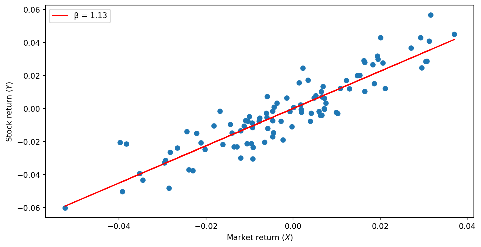
From Correlation to Linear Regression
Correlation tells us whether two variables move together. Linear regression goes further: it finds the best-fitting line.
\[Y = \alpha + \beta X + \epsilon\]
\(\alpha\) (alpha) = intercept (where the line crosses the y-axis)
\(\beta\) (beta) = slope (how much \(Y\) changes when \(X\) increases by 1)
\(\epsilon\) (epsilon) = error term (the part we can’t explain)
The sign of \(\beta\) matches the sign of correlation:
This is the foundation of machine learning: finding relationships in data. sklearn (scikit-learn) is the library we’ll use for ML throughout this course.
Part II: Calculus
Functions: A Quick Reminder
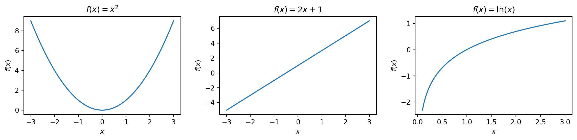
A function takes an input and produces an output: \(f(x) = x^2\)
Input \(x = 3\) → Output \(f(3) = 9\)
Input \(x = -2\) → Output \(f(-2) = 4\)
We can visualize functions by plotting input (\(x\)-axis) against output (\(y\)-axis):
In ML, we’ll work with functions that measure error—and we’ll want to find the input that makes the error as small as possible.
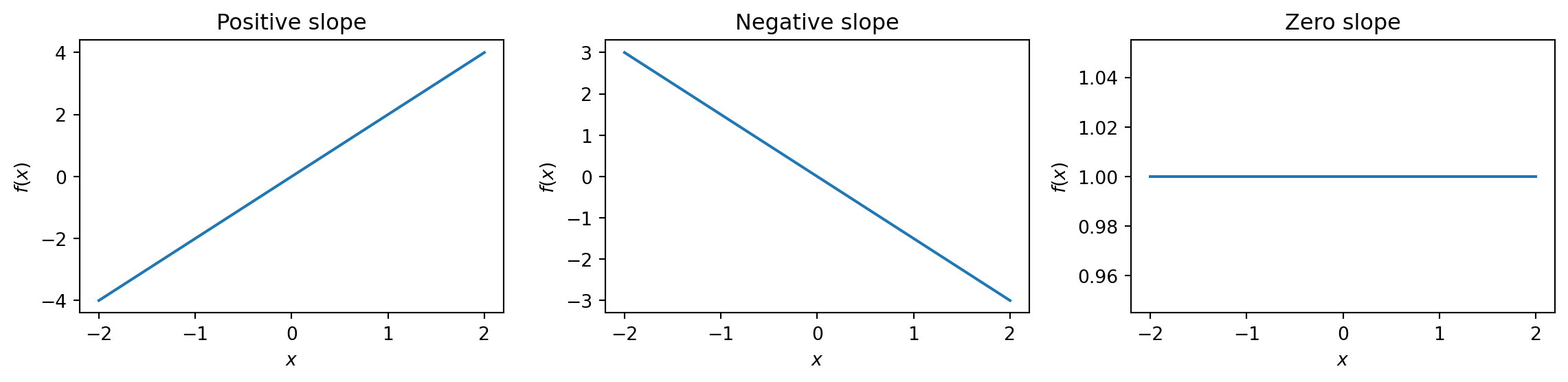
Slope: Rise Over Run
For a straight line, the slope tells you how steep it is:
But what about curves? The slope is different at every point…
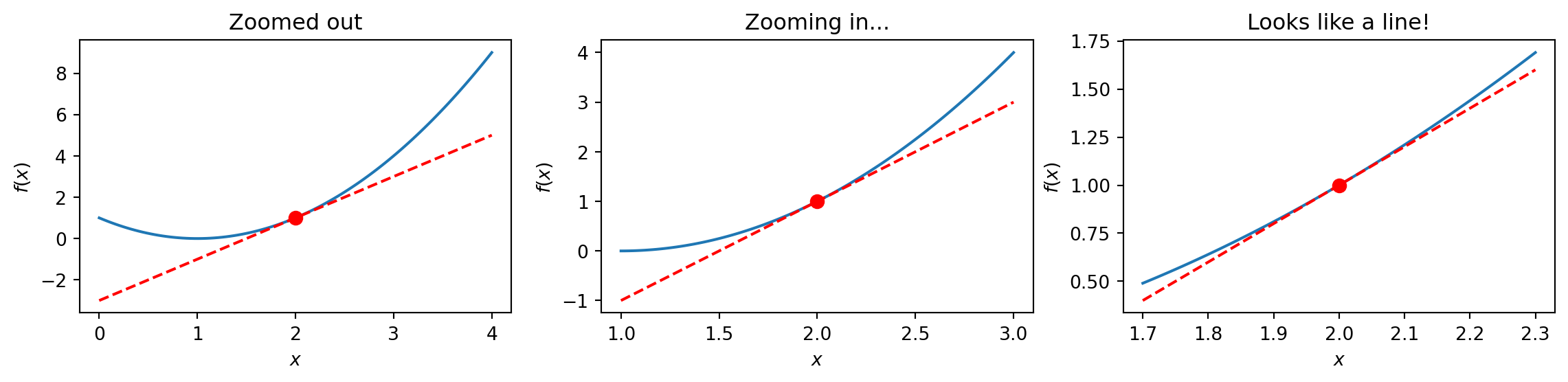
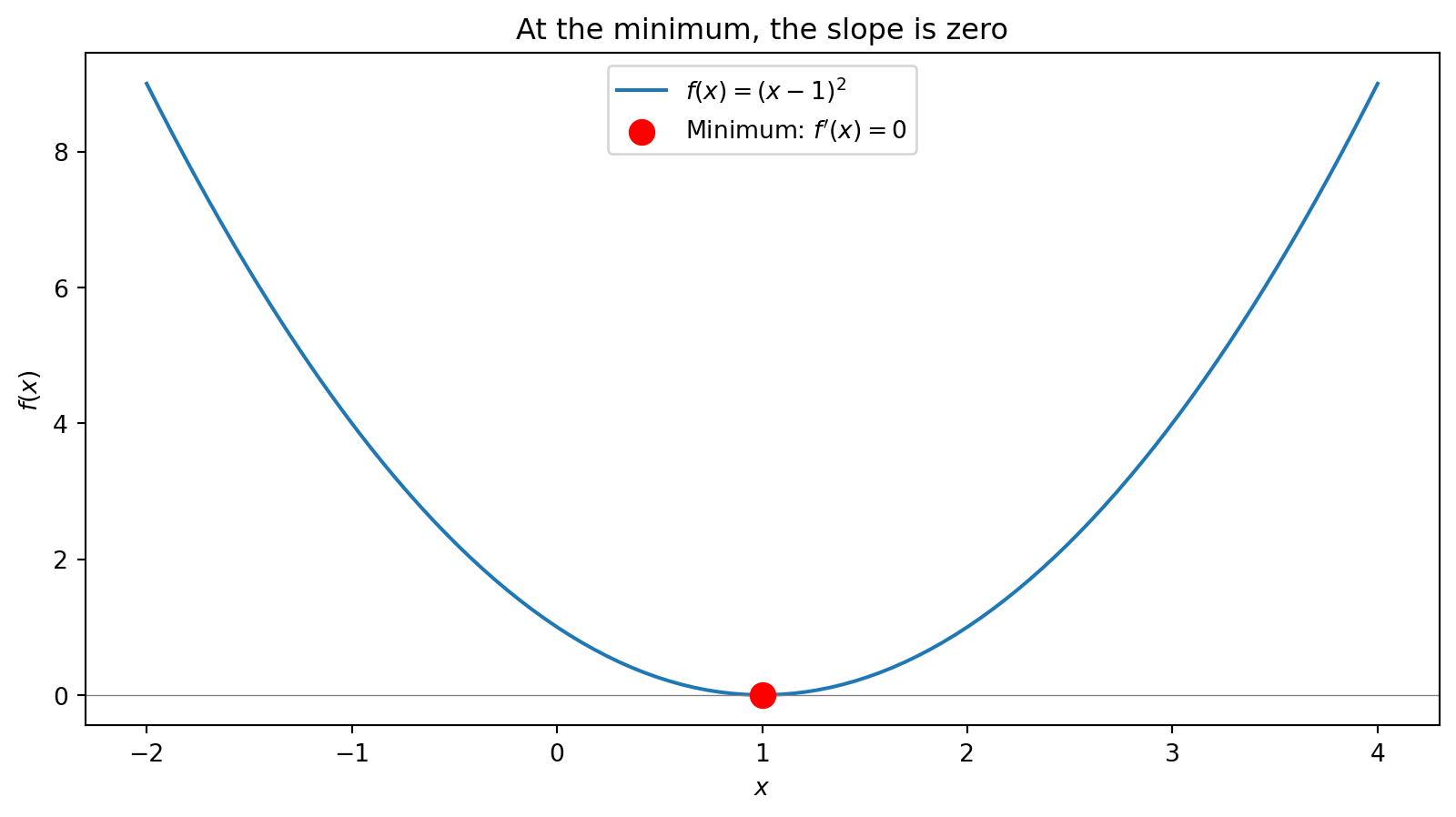
Derivatives: Slope at a Point
The derivative is the slope of a curve at a specific point—the “instantaneous” rate of change.
Imagine zooming in on a curve until it looks like a straight line. The slope of that line is the derivative.
At \(x = 2\), the curve \(f(x) = (x-1)^2\) has slope 2. We write: \(f'(2) = 2\).
Derivative Notation
Several notations mean the same thing—the derivative of \(f\) with respect to \(x\):
\[f'(x) = \frac{df}{dx} = \frac{d}{dx}f(x)\]
\(f'(x)\) — “f prime of x”
\(\frac{df}{dx}\) — “df dx” (Leibniz notation, emphasizes “change in \(f\) per change in \(x\)”)
What the derivative tells you:
\(f'(x) > 0\): function is increasing at \(x\)
\(f'(x) < 0\): function is decreasing at \(x\)
\(f'(x) = 0\): function is flat at \(x\)
Why We Care: Finding Extrema
An extremum (plural: extrema) is a minimum or maximum of a function.
At an extremum, the function is flat—it’s neither increasing nor decreasing. That means the derivative is zero.
This is the key insight: To find where a function is minimized (or maximized), find where its derivative equals zero.
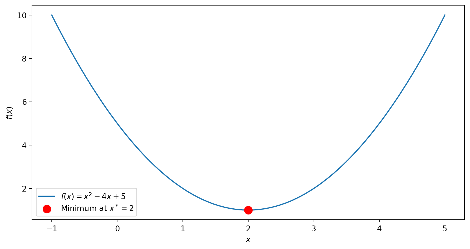
Finding Minima: The Recipe
To find the minimum of \(f(x)\):
Take the derivative \(f'(x)\)
Set \(f'(x) = 0\) and solve for \(x\)
You won’t be computing derivatives by hand in this course—computers handle that. But you need to understand the logic: the minimum is where the slope is zero.
Why this matters for ML: In machine learning, we define a loss function that measures error. Training a model means finding the parameters that minimize that loss—finding where the slope is zero.
Functions of Multiple Variables
So far we’ve looked at functions of one variable: \(f(x)\). But what if a function depends on two (or more) variables?
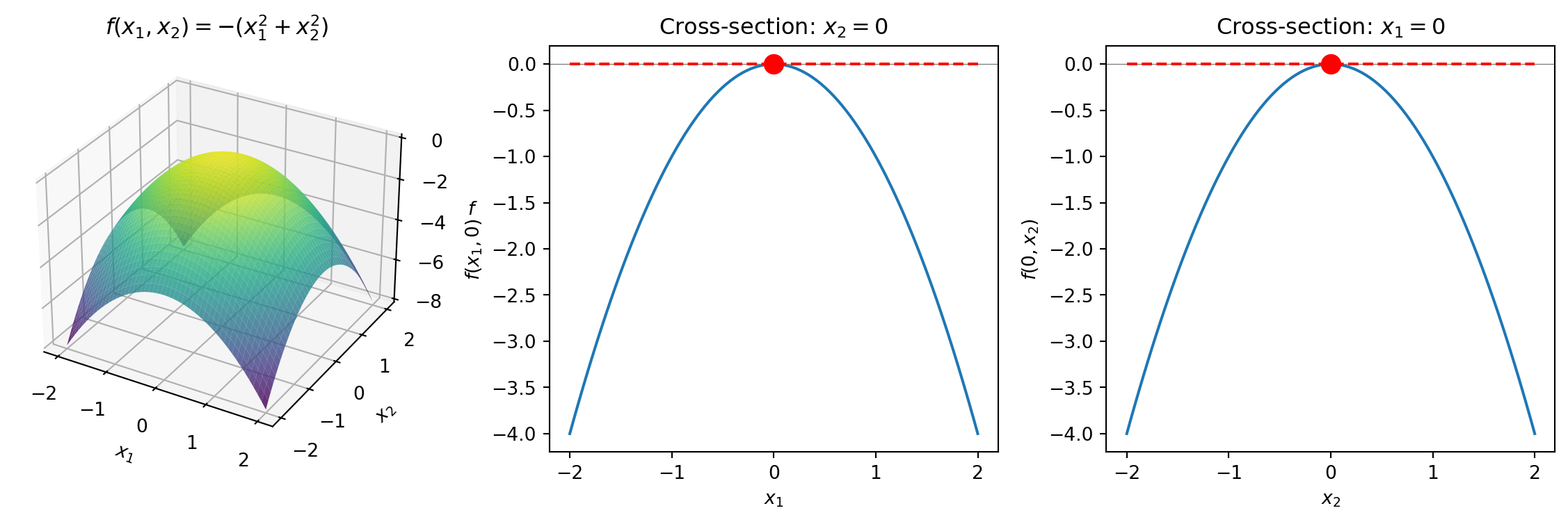
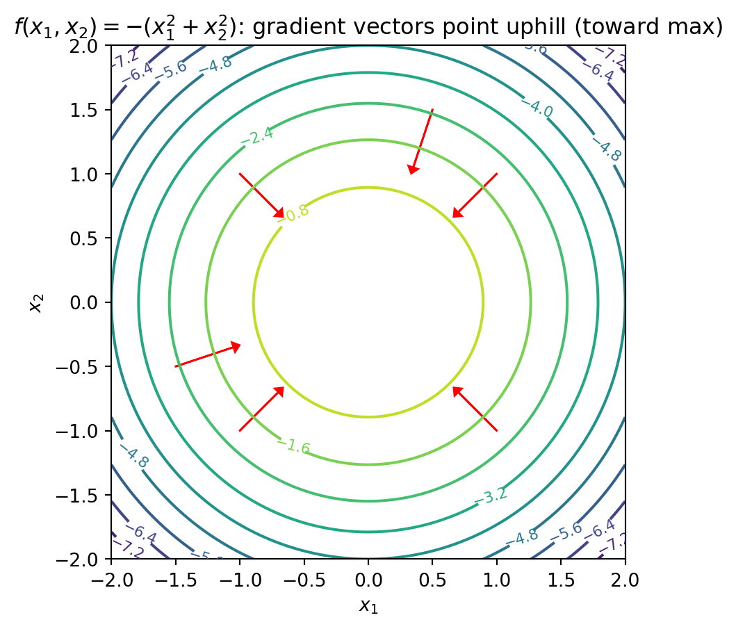
\[f(x_1, x_2) = -(x_1^2 + x_2^2)\]
This function takes two inputs and produces one output. We can visualize it as a surface in 3D:
The maximum is at the origin \((0, 0)\)—the top of the “dome.” In both cross-sections, the tangent line is flat (slope = 0) at the extremum.
Partial Derivatives: Slope in One Direction
How do we find the extremum of a function with multiple variables?
We ask: if I move in just the \(x_1\) direction (holding \(x_2\) fixed), what’s the slope? That’s the partial derivative with respect to \(x_1\). We can do the same for \(x_2\).
Look back at our cross-sections: each one shows the slope in one direction. At the top of the dome, both cross-sections are flat—the slope is zero in every direction.
At an extremum, all partial derivatives are zero. The surface is flat no matter which direction you look. This is what optimization algorithms search for.
Part III: Linear Algebra
Why Linear Algebra?
We’ve seen that derivatives are slopes—and slopes are lines. Linear relationships are easy to work with: easy to compute, easy to optimize, easy to interpret.
Vectors and matrices let us extend this to multiple dimensions:
One variable
Multiple variables
Derivative \(f'(x)\)
Gradient \(\nabla f\) (vector of partial derivatives)
The structure is the same—we just stack things into vectors and matrices. Instead of writing \(n\) separate equations, we write one matrix equation. This is the language of machine learning.
Vectors
A vector is an ordered list of numbers. We write vectors in bold: \(\mathbf{x}\)
We say \(\mathbf{x} \in \mathbb{R}^n\) meaning “\(\mathbf{x}\) is a vector of \(n\) real numbers.”
For matrix multiplication, think of a vector as an \((n \times 1)\) matrix—a matrix with \(n\) rows and 1 column.
# Vectors in numpyx = np.array([1, 2, 3, 4, 5])print(f"x = {x}")print(f"x has {len(x)} elements")print(f"x[0] = {x[0]}") # First element (Python is 0-indexed)
x = [1 2 3 4 5]
x has 5 elements
x[0] = 1
Matrices
A matrix is a 2D array of numbers. We write matrices in bold capitals: \(\mathbf{X}\)
Matrix multiplication is NOT commutative. With scalars \(a,b\in\mathbb{R}\), \(a \times b = b \times a\). But with matrices, \(\mathbf{A}\mathbf{B} \neq \mathbf{B}\mathbf{A}\) in general. The order matters!
The identity matrix\(\mathbf{I}\) has 1s on the diagonal and 0s everywhere else. It’s the matrix analogue of multiplying by 1:
Matrix inverse: For square matrices, under the right conditions, we can find an inverse \(\mathbf{A}^{-1}\) such that \(\mathbf{A}^{-1}\mathbf{A} = \mathbf{A}\mathbf{A}^{-1} = \mathbf{I}\). This lets us “undo” multiplication—analogous to division for scalars.
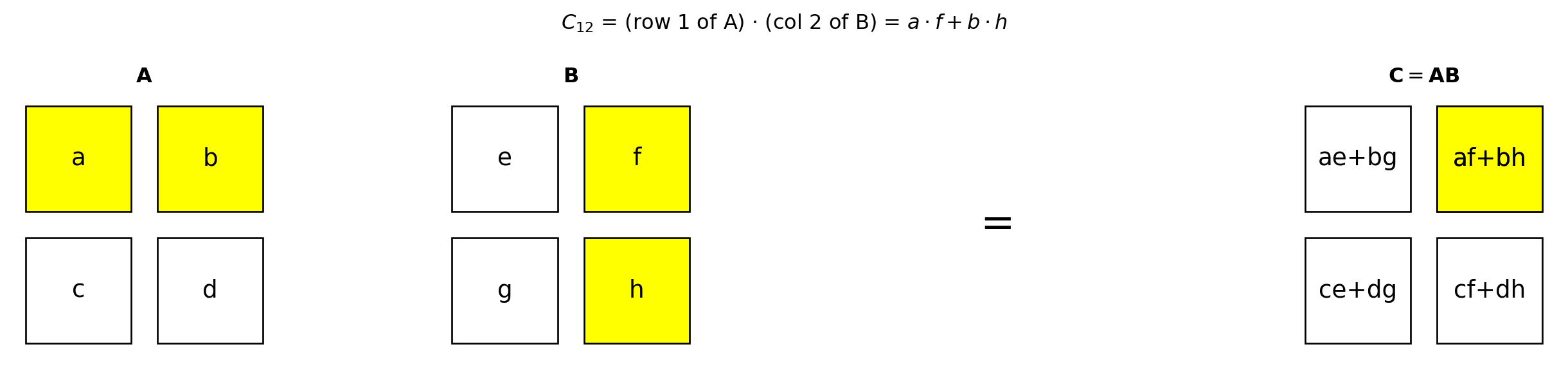
Advanced: How matrix multiplication works
Each element of the output is a dot product. Specifically, element \((i, j)\) of \(\mathbf{C} = \mathbf{A}\mathbf{B}\) is the dot product of row \(i\) of \(\mathbf{A}\) with column \(j\) of \(\mathbf{B}\):
\[C_{ij} = \sum_{k=1}^{n} A_{ik} B_{kj}\]
In Python, use @ for matrix multiplication and .T for transpose:
The ordinary least squares (OLS) solution is: \(\hat{\boldsymbol{\beta}} = (\mathbf{X}'\mathbf{X})^{-1}\mathbf{X}'\mathbf{y}\)
Advanced: Where does the OLS formula come from?
Start with \(\mathbf{y} = \mathbf{X}\boldsymbol{\beta} + \boldsymbol{\epsilon}\). In expectation, \(\boldsymbol{\epsilon}\) averages to zero, so we want to solve \(\mathbf{y} = \mathbf{X}\boldsymbol{\beta}\) for \(\boldsymbol{\beta}\).
We’d like to “divide by \(\mathbf{X}\)” but \(\mathbf{X}\) is \((n \times p)\)—not square, so not invertible!
The trick: premultiply both sides by \(\mathbf{X}'\) to make it square: \[\begin{align*}
\mathbf{X}'\mathbf{y} &= \mathbf{X}'\mathbf{X}\boldsymbol{\beta}
\end{align*}\]
Now \(\mathbf{X}'\mathbf{X}\) is \((p \times p)\)—square and invertible. Premultiply both sides by \((\mathbf{X}'\mathbf{X})^{-1}\): \[\begin{align*}
(\mathbf{X}'\mathbf{X})^{-1}\mathbf{X}'\mathbf{y} &= (\mathbf{X}'\mathbf{X})^{-1}\mathbf{X}'\mathbf{X}\boldsymbol{\beta} \\
(\mathbf{X}'\mathbf{X})^{-1}\mathbf{X}'\mathbf{y} &= \mathbf{I}\boldsymbol{\beta} \\
\boldsymbol{\beta} &= (\mathbf{X}'\mathbf{X})^{-1}\mathbf{X}'\mathbf{y}
\end{align*}\]
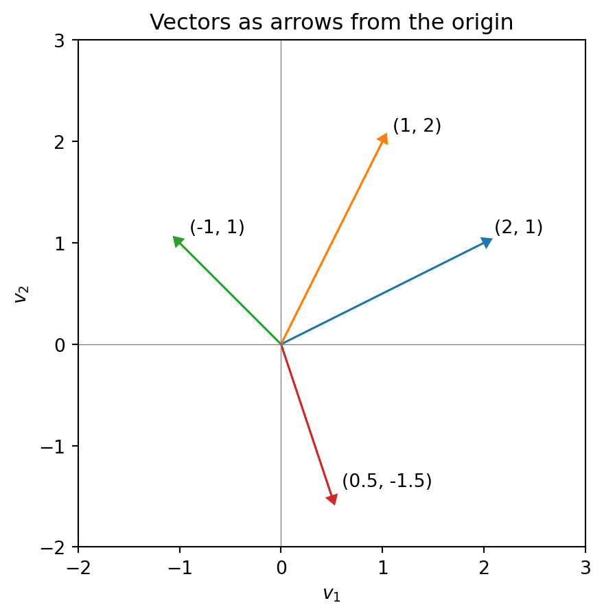
Vectors Have Direction
A vector in \(\mathbb{R}^2\) is just two numbers: \(\mathbf{v} = \begin{bmatrix} v_1 \\ v_2 \end{bmatrix}\)
But we can also think of it as an arrow that points somewhere:
The vector \(\begin{bmatrix} 2 \\ 1 \end{bmatrix}\) points “2 units right and 1 unit up.”
Linear Algebra Application: The Gradient
The gradient is the vector of all partial derivatives:
OLS has a nice closed-form solution: we can write down a formula and compute the answer directly.
Most ML methods don’t have this luxury. For neural networks, random forests, and many other models, there’s no formula—we have to search for the optimum iteratively using algorithms like gradient descent. That’s why we spend so much time on optimization in this course!
Everything we covered today is a building block for this: - Statistics tells us what we’re estimating - Calculus tells us how to find minima - Linear algebra gives us compact notation - Optimization ties it all together
VS Code is not the only option—you could use PyCharm, Jupyter notebooks directly, or even a plain text editor. But VS Code is free, widely used in industry, and works well for this course.