RSM338: Machine Learning in Finance

Lecture 9: Neural Networks & Deep Learning | March 18–19, 2026

Kevin Mott

Rotman School of Management

Today’s Goal

Today we introduce the last and most flexible model in the course: neural networks. To get there, we need to reconnect to a framework from Lecture 5 that has been quietly running behind every model we’ve studied since.

Today’s roadmap:

Deep learning = regression: Connecting back to the Lecture 5 framework
Opening the hood: What’s inside a neural network?
The universal approximation theorem: Why neural networks can represent any function
Training neural networks: Loss, backpropagation, optimizers, and the training loop
Regularization: Preventing overfitting in overparameterized models
Demo: Building a neural network in PyTorch
Beyond feed-forward: CNNs, autoencoders, RNNs, transformers, and GANs

Part I: Deep Learning = Regression

The Regression Toolkit (Lecture 5 Recap)

In Lecture 5 we generalized OLS into a “choose your ingredients” framework. Here was the slide:

\[\hat{\theta} = \arg\min_{\theta} \left\{ \underbrace{\sum_{i=1}^{n} \mathcal{L}(y_i, f_\theta(\mathbf{x}_i))}_{\text{loss function}} + \underbrace{\lambda \cdot \text{Penalty}(\theta)}_{\text{regularization}} \right\}\]

where \(f_\theta\) is the prediction function (parameterized by \(\theta\)), \(\mathcal{L}\) is the loss measuring how wrong our predictions are, and \(\lambda \cdot \text{Penalty}(\theta)\) is an optional regularization term that penalizes complex models.

Component	OLS Choice	Alternatives
Function \(f_\theta\)	Linear: \(\mathbf{x}^\top \boldsymbol{\beta}\)	Polynomial, tree, neural network
Loss \(\mathcal{L}\)	Squared error	Absolute error, Huber, cross-entropy
Penalty	None (\(\lambda = 0\))	Ridge (L2), Lasso (L1), Elastic Net

At the time, we said “non-linear \(f\) comes in later lectures.” Every lecture since has been filling in a specific choice for \(f_\theta\) from the “Alternatives” column — we just didn’t always call it that.

How Every Model Fits the Framework

Here’s where each model sits in that table:

Lecture	Model	What \(f_\theta(\mathbf{x})\) is	Parameters \(\theta\)
5	Linear regression	\(\mathbf{x}^\top \boldsymbol{\beta}\)	Slopes and intercept
5	Ridge / Lasso	\(\mathbf{x}^\top \boldsymbol{\beta}\) (with penalty)	Slopes and intercept
7	Logistic regression	\(\sigma(\mathbf{x}^\top \mathbf{w})\)	Weights and bias
8	Decision trees / ensembles	Piecewise-constant regions	Split rules and leaf values

In every case, the parameters \(\theta\) had clear interpretations. You could look at a regression coefficient and say “\(\beta_3 = 0.5\) means a one-unit increase in \(X_3\) is associated with a 0.5-unit increase in \(Y\).” Even tree splits are interpretable: “if momentum > 0.02, go left.”

The Neural Network as \(f_\theta\)

Today we add one more row to the table:

Lecture	Model	What \(f_\theta(\mathbf{x})\) is	Parameters \(\theta\)
9	Neural network	A composition of layers	Thousands (millions? billions?) of weights

A neural network is just another choice of \(f_\theta\) — same loss functions, same regularization ideas. What’s different:

\(f_\theta\) is built by composing many simple operations — layer after layer of weighted sums and nonlinear transformations
\(\theta\) contains thousands or millions of weights and biases
The parameters have no individual interpretation — you cannot look at weight #4,817 and say what it “means”
The model is a black box: features go in, predictions come out

Why Give Up Interpretability?

If we can’t interpret the parameters, why would we use a neural network?

Because the other models on our list have structural limitations:

Linear regression can only learn linear relationships
Logistic regression can only learn linear decision boundaries
Decision trees partition the feature space into rectangles
Even Random Forests and XGBoost are combinations of piecewise-constant functions

Neural networks trade interpretability for flexibility:

By composing many layers, they can approximate essentially any continuous function (we’ll make this precise later)
The cost: you lose the ability to explain why the model makes a particular prediction
Worth it when prediction accuracy matters more than explanation (fraud detection, algorithmic trading)

Part II: Opening the Hood

A Single Neuron

The building block of every neural network is a neuron (also called a unit or node). A single neuron does two things:

Compute a weighted sum of its inputs, plus a bias term
Apply a nonlinear function (called an activation function) to the result

\[a = g\!\left(\sum_{j=1}^{p} w_j x_j + b\right) = g(\mathbf{w}^\top \mathbf{x} + b)\]

where:

\(x_1, x_2, \ldots, x_p\) are the inputs (our features)
\(w_1, w_2, \ldots, w_p\) are the weights — how much each input contributes
\(b\) is the bias — an offset (like an intercept)
\(g(\cdot)\) is the activation function — introduces nonlinearity

The weighted sum \(\mathbf{w}^\top \mathbf{x} + b\) should look familiar: it’s the same linear combination from logistic regression. The activation function \(g\) is what makes this more than a linear model.

A Neuron Is Logistic Regression

If we choose the sigmoid as our activation function, a single neuron is exactly logistic regression:

\[a = \sigma(\mathbf{w}^\top \mathbf{x} + b) = \frac{1}{1 + e^{-(\mathbf{w}^\top \mathbf{x} + b)}}\]

This is the same formula from the classification lecture. One neuron with a sigmoid activation = logistic regression. A neural network is what happens when we stack many of these neurons together.

If we choose no activation function at all (the “identity” activation, \(g(z) = z\)), a single neuron is just linear regression: \(\hat{y} = \mathbf{w}^\top \mathbf{x} + b\).

So neural networks are not a departure from what we’ve learned — they’re a generalization. The models we already know are special cases.

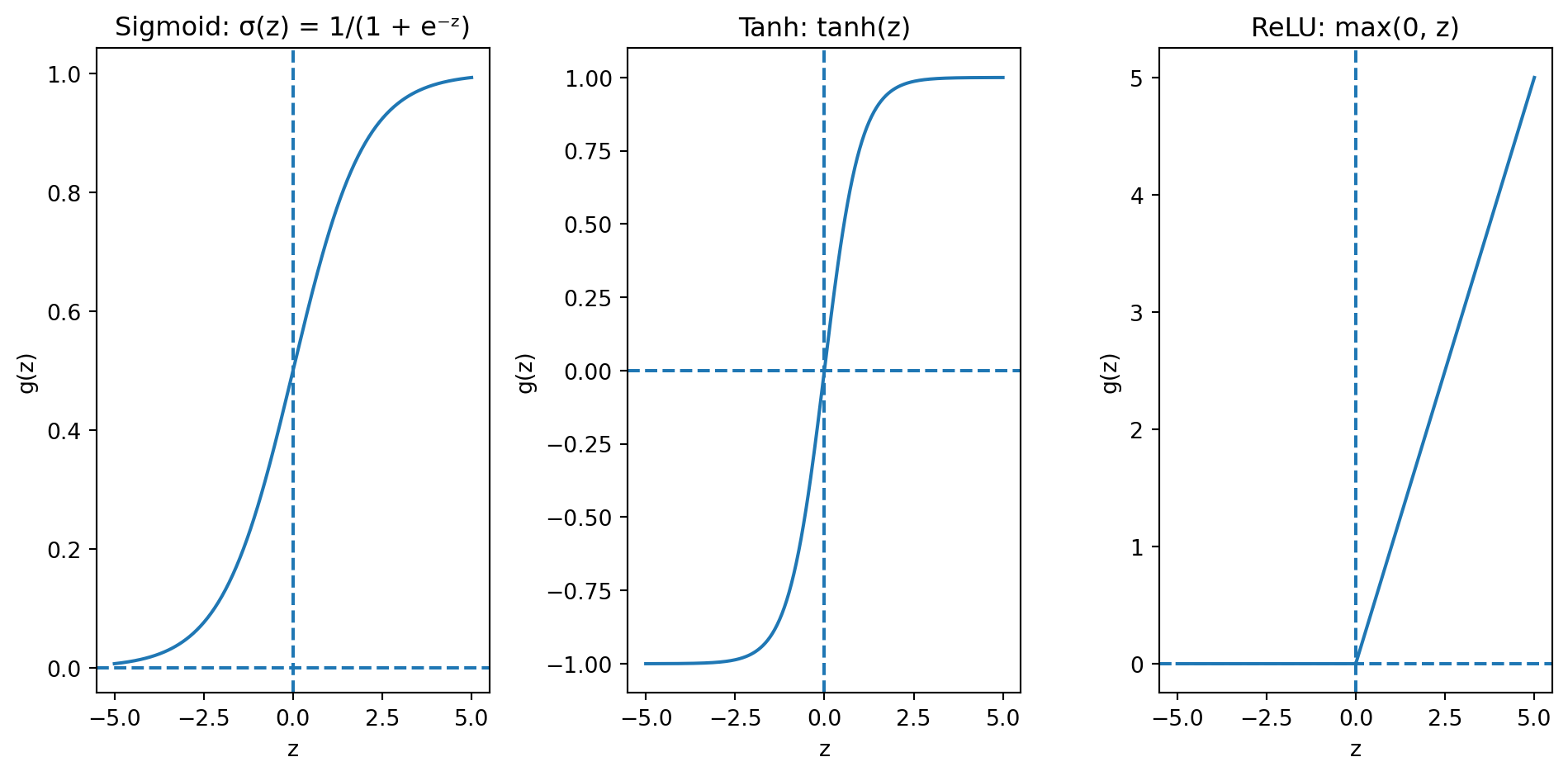
Activation Functions

The activation function \(g\) controls what kind of nonlinearity each neuron introduces. Here are the most common choices:

Sigmoid (\(\sigma\)): Squashes to (0, 1). Used for binary classification output layers. Suffers from vanishing gradients in deep networks.
Tanh: Squashes to (−1, 1). Centred at zero (better for hidden layers). Still has vanishing gradients.
ReLU (Rectified Linear Unit): \(g(z) = \max(0, z)\). The modern default. Simple, fast, avoids vanishing gradients for positive inputs. Downside: outputs exactly zero for negative inputs (“dead neurons”).

Why Activation Functions Matter

Without activation functions, stacking layers doesn’t help. Suppose we have two layers of linear transformations:

\[\text{Layer 1: } \mathbf{h} = \mathbf{W}_1 \mathbf{x} + \mathbf{b}_1\] \[\text{Layer 2: } \hat{y} = \mathbf{W}_2 \mathbf{h} + \mathbf{b}_2\]

Substituting:

\[\hat{y} = \mathbf{W}_2 (\mathbf{W}_1 \mathbf{x} + \mathbf{b}_1) + \mathbf{b}_2 = \underbrace{(\mathbf{W}_2 \mathbf{W}_1)}_{\mathbf{W}'} \mathbf{x} + \underbrace{(\mathbf{W}_2 \mathbf{b}_1 + \mathbf{b}_2)}_{\mathbf{b}'}\]

This is still a linear function of \(\mathbf{x}\). No matter how many linear layers we stack, the result is always equivalent to a single linear transformation. The depth buys us nothing.

Activation functions break this collapse. When we insert \(g\) between layers:

\[\hat{y} = \mathbf{W}_2 \, g(\mathbf{W}_1 \mathbf{x} + \mathbf{b}_1) + \mathbf{b}_2\]

the \(g\) prevents us from simplifying. Each layer now genuinely transforms the representation. This is why depth matters — but only with nonlinear activations.

From One Neuron to a Layer

A layer is a collection of neurons that all receive the same inputs but have different weights. With \(d\) neurons and \(p\) input features, the whole layer is one matrix operation:

\[\mathbf{h} = g(\mathbf{W}\mathbf{x} + \mathbf{b})\]

where:

\(\mathbf{W}\) is a \(d \times p\) weight matrix — row \(k\) contains the weights for neuron \(k\)
\(\mathbf{b}\) is a \(d \times 1\) bias vector — one bias per neuron
\(g\) is applied element-wise to each neuron’s output
\(\mathbf{h}\) is the \(d \times 1\) output vector — one value per neuron

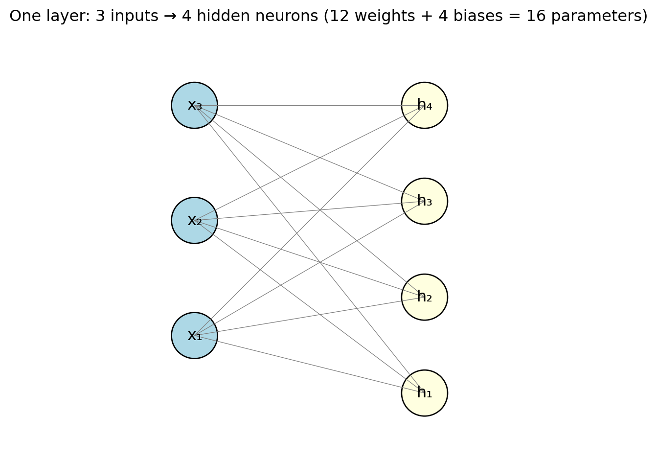
Each line in the diagram represents one weight. With 3 inputs and 4 neurons, that’s \(3 \times 4 = 12\) weights plus 4 biases = 16 parameters. Already more than the 4 parameters in a 3-variable linear regression.

Stacking Layers: The Feed-Forward Network

A feed-forward neural network (or multilayer perceptron / MLP) stacks layers — each layer’s output feeds into the next:

\[\mathbf{h}^{(1)} = g\!\left(\mathbf{W}^{(1)} \mathbf{x} + \mathbf{b}^{(1)}\right)\] \[\mathbf{h}^{(2)} = g\!\left(\mathbf{W}^{(2)} \mathbf{h}^{(1)} + \mathbf{b}^{(2)}\right)\] \[\hat{y} = \mathbf{W}^{(3)} \mathbf{h}^{(2)} + \mathbf{b}^{(3)}\]

\(\mathbf{h}^{(\ell)}\) = hidden layer — “hidden” because we never observe these values directly
The final layer is the output layer, producing the prediction

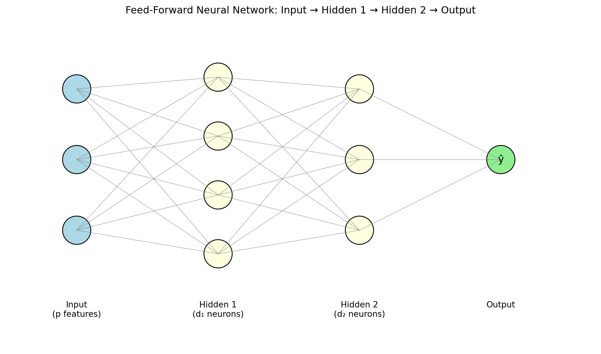
Information flows one direction: input → hidden layers → output (no loops or feedback)
Depth = number of hidden layers. Modern “deep learning” models may have dozens or hundreds.

The Parameter Explosion

Let’s count parameters for a concrete example. Suppose we have:

\(p = 10\) input features
Hidden layer 1: 64 neurons
Hidden layer 2: 32 neurons
Output: 1 neuron (regression) or \(K\) neurons (classification)

Connection	Weights	Biases	Total
Input → Hidden 1	\(10 \times 64 = 640\)	64	704
Hidden 1 → Hidden 2	\(64 \times 32 = 2{,}048\)	32	2,080
Hidden 2 → Output	\(32 \times 1 = 32\)	1	33
Total			2,817

10 features, two modest hidden layers → nearly 3,000 parameters (vs. 11 for linear regression)
ResNet-50 (image classifier): 25 million parameters
Large language models: billions
Parameters typically far exceed training observations — a regime where OLS wouldn’t even have a unique solution

The Output Layer

The final layer of the network depends on the task:

Regression (predicting a continuous value like returns):

One output neuron with no activation (identity): \(\hat{y} = \mathbf{w}^\top \mathbf{h} + b\)
The output can be any real number

Binary classification (predicting default / no default):

One output neuron with sigmoid activation: \(\hat{y} = \sigma(\mathbf{w}^\top \mathbf{h} + b)\)
The output is a probability between 0 and 1
Same as logistic regression’s output, but \(\mathbf{h}\) is a learned representation instead of raw features

Multi-class classification (predicting which of \(K\) sectors):

\(K\) output neurons with softmax activation: \[\hat{y}_k = \frac{e^{z_k}}{\sum_{j=1}^{K} e^{z_j}}\]
Outputs sum to 1 — a probability distribution over classes

Hidden layers learn a useful representation; the output layer translates it into the prediction format we need.

Putting It All Together: The Full Picture

A neural network is just a function \(f_\theta(\mathbf{x})\) that we plug into the same regression framework from Lecture 5:

\[\hat{\theta} = \arg\min_{\theta} \left\{ \sum_{i=1}^{n} \mathcal{L}\!\left(y_i, \; f_\theta(\mathbf{x}_i)\right) + \lambda \cdot \text{Penalty}(\theta) \right\}\]

What makes it different:

\(f_\theta\) is a composition of layers: weighted sums → activations → weighted sums → activations → \(\cdots\) → output
\(\theta\) = all the weights and biases across all layers (thousands or millions of numbers)
There is no closed-form solution. We must use iterative optimization (gradient descent) to find the best \(\theta\)
The parameters \(\theta\) have no individual interpretation — the model is a black box

The loss \(\mathcal{L}\), the regularization penalty, the train/test split, cross-validation — all the machinery from earlier lectures carries over. The only new ingredient is the architecture of \(f_\theta\).

Part III: The Universal Approximation Theorem

Can Neural Networks Actually Learn Anything?

How flexible is a neural network, exactly? Could it represent any relationship?

Yes — with a caveat.

The Universal Approximation Theorem (Cybenko, 1989; Hornik, 1991):

A feed-forward neural network with a single hidden layer containing a sufficient number of neurons can approximate any continuous function on a compact domain to arbitrary accuracy.

In plain language: given enough neurons, a one-hidden-layer network can get as close as you want to any smooth function.

What the Theorem Promises

The theorem says a wide enough network can represent extremely complex functions:

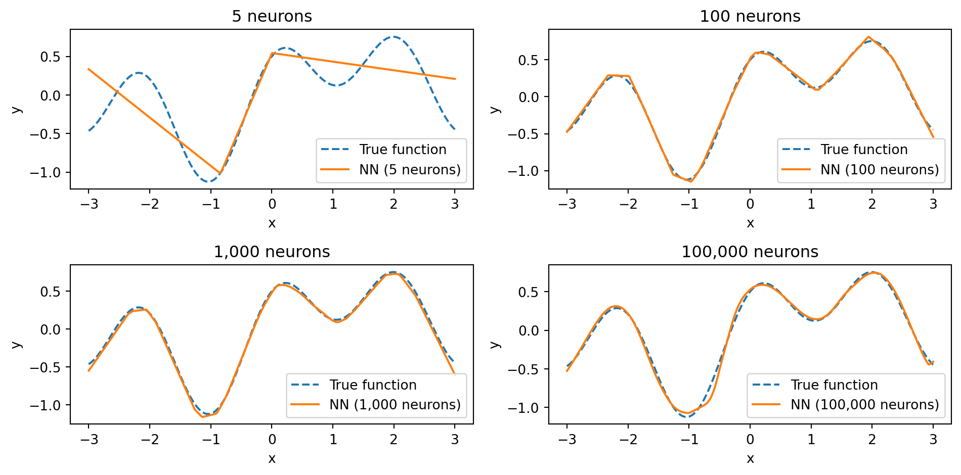
With 5 neurons, the network captures only the broad shape. With 100, it gets most of the detail. With 1,000 and 100,000 neurons, the fit becomes nearly perfect — the network has enough capacity to match every wiggle of the true function. The universal approximation theorem guarantees that we can get as close as we want — if we use enough neurons.

What the Theorem Does NOT Promise

The theorem is an existence result, not a practical guarantee. It says a solution exists, not that we can find it.

It doesn’t promise:

That gradient descent will find the right weights. The loss landscape of a neural network is non-convex — it has many local minima and saddle points. The optimization could get stuck.
How many neurons you need. The theorem says “a sufficient number,” but that number could be impractically large.
That the network will generalize. A network with enough parameters can memorize the training data perfectly (just like a high-degree polynomial). The theorem says nothing about performance on new data.
That one hidden layer is the best architecture. The theorem proves one wide layer is enough, but in practice, deeper networks with fewer neurons per layer are more efficient. They can represent certain functions with far fewer total parameters than a single wide layer would need.

This last point is the practical motivation for deep learning. Depth is not about theoretical power (one layer is enough) — it’s about efficiency and learning useful representations at each level.

Part IV: Training Neural Networks

The Training Problem

We need to find the parameters \(\theta\) (all weights and biases) that minimize the loss:

\[\theta^* = \arg\min_{\theta} \frac{1}{n} \sum_{i=1}^{n} \mathcal{L}\!\left(y_i, \; f_\theta(\mathbf{x}_i)\right)\]

Linear regression: closed-form solution
Neural network: no closed-form — the loss is non-convex (many bumps and valleys) because of nonlinear activations

We solve it with gradient descent: start with random weights, compute the gradient, step in the opposite direction:

\[\theta_{t+1} = \theta_t - \eta \, \nabla_\theta \mathcal{L}\]

where \(\eta\) (eta) is the learning rate — how large a step we take.

Loss Functions

Same losses from earlier lectures — they carry over directly.

Regression:

\[\mathcal{L}_{\text{MSE}} = \frac{1}{n}\sum_{i=1}^{n}(y_i - \hat{y}_i)^2\]

Mean squared error — same as OLS.

Binary classification:

\[\mathcal{L}_{\text{BCE}} = -\frac{1}{n}\sum_{i=1}^{n}\left[y_i \log(\hat{y}_i) + (1 - y_i)\log(1 - \hat{y}_i)\right]\]

Binary cross-entropy — same as logistic regression. Heavily penalizes confident wrong predictions.

Multi-class classification (\(K\) classes):

\[\mathcal{L}_{\text{CE}} = -\frac{1}{n}\sum_{i=1}^{n}\sum_{k=1}^{K} y_{ik} \log(\hat{y}_{ik})\]

where \(y_{ik} = 1\) if observation \(i\) belongs to class \(k\) and 0 otherwise.

Backpropagation: How Does the Network Learn?

With thousands of parameters, how do we compute the gradient \(\nabla_\theta \mathcal{L}\)?

Backpropagation (Rumelhart, Hinton & Williams, 1986) computes the gradient of the loss with respect to every weight. It works because a neural network is a nested composition of functions. For a 3-layer network:

\[\begin{align*} \mathbf{h}^{(1)} &= g\!\left(\mathbf{W}^{(1)} \mathbf{x} + \mathbf{b}^{(1)}\right) \\ \mathbf{h}^{(2)} &= g\!\left(\mathbf{W}^{(2)} \mathbf{h}^{(1)} + \mathbf{b}^{(2)}\right) \\ \hat{y} &= \mathbf{W}^{(3)} \mathbf{h}^{(2)} + \mathbf{b}^{(3)} \end{align*}\]

Substituting, the prediction is a nested composition:

\[\hat{y} = f^{(3)}\!\Big(\; f^{(2)}\!\Big(\; f^{(1)}(\mathbf{x})\;\Big)\;\Big)\]

where \(f^{(\ell)}(\cdot) = g(\mathbf{W}^{(\ell)}(\cdot) + \mathbf{b}^{(\ell)})\). The chain rule differentiates through each layer:

\[\frac{\partial \mathcal{L}}{\partial \mathbf{W}^{(1)}} = \underbrace{\frac{\partial \mathcal{L}}{\partial \hat{y}}}_{\text{output}} \cdot \underbrace{\frac{\partial \hat{y}}{\partial \mathbf{h}^{(2)}}}_{\text{layer 3}} \cdot \underbrace{\frac{\partial \mathbf{h}^{(2)}}{\partial \mathbf{h}^{(1)}}}_{\text{layer 2}} \cdot \underbrace{\frac{\partial \mathbf{h}^{(1)}}{\partial \mathbf{W}^{(1)}}}_{\text{layer 1}}\]

Each factor involves only one layer’s local operation — easy to compute
Forward pass: compute the loss
Backward pass: multiply these local derivatives from right to left
Weights that contributed more to the error get larger updates
Modern frameworks (PyTorch, JAX) do this automatically

The Vanishing Gradient Problem

The chain rule multiplies many factors together. If each is small, the gradient shrinks exponentially:

If each layer’s gradient is 0.25, then after 4 layers: \(0.25^4 \approx 0.004\) — nearly zero
Early layers barely learn because the error signal is too weak by the time it reaches them

Why this happens with sigmoid/tanh: Their gradients are always < 1 (sigmoid’s max is 0.25), so the chain rule multiplies many small numbers together.

Why ReLU helps: Its gradient is either 0 or 1. For positive inputs, the gradient passes through unchanged — no shrinkage.

Stochastic Gradient Descent and Mini-Batches

Standard gradient descent uses the entire training set at each step — slow with millions of observations.

Stochastic Gradient Descent (SGD) uses a small random subset (a mini-batch) instead:

\[\theta_{t+1} = \theta_t - \eta \, \nabla_\theta \mathcal{L}_{\text{batch}}\]

The mini-batch gradient is a noisy estimate of the true gradient — on average, it points the right way
The noise actually helps: it can bounce the optimizer out of shallow local minima
Common batch sizes: 32, 64, 128, 256
Smaller batches → more noise, slower convergence
Larger batches → smoother gradients, more memory

Epochs

An epoch is one complete pass through the entire training set.

If you have 10,000 training observations and a batch size of 100, each epoch consists of 100 mini-batch updates. After one epoch, every observation has been used exactly once.

Training typically runs for many epochs — the optimizer sees the same data repeatedly, refining the weights each time.

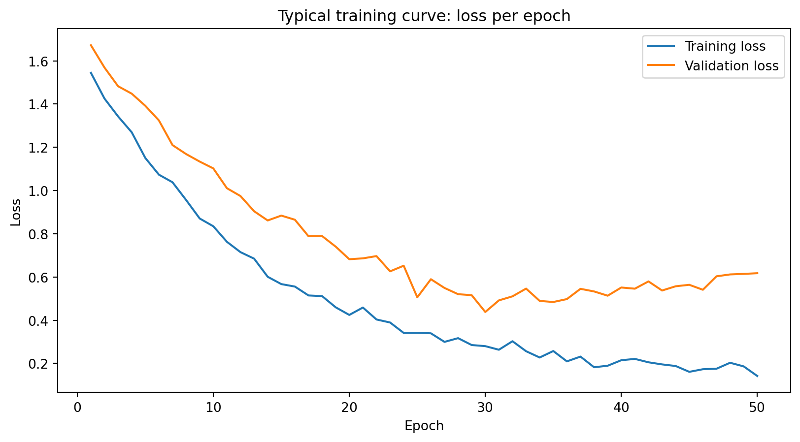
Training loss decreases steadily. Validation loss decreases initially, then starts to increase — the model begins overfitting. The gap between the curves signals that the model is memorizing training data rather than learning generalizable patterns.

The Learning Rate

The learning rate \(\eta\) is usually the first hyperparameter to tune when training a neural network.

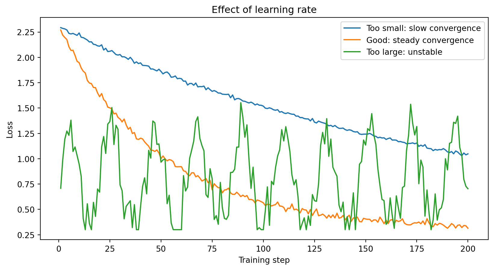
Too small: The model learns very slowly. You might need thousands of epochs to converge — wasteful and sometimes impractical.

Too large: The model overshoots and bounces around, never settling into a good minimum. The loss oscillates or even diverges.

Just right: The loss decreases steadily and converges to a low value.

Typical starting values: \(\eta = 0.001\) for Adam optimizer, \(\eta = 0.01\) for SGD. Often reduced during training (learning rate scheduling).

Optimizers: Beyond Basic Gradient Descent

Plain SGD uses the same learning rate for every parameter and doesn’t account for the history of past gradients. Modern optimizers improve on this.

SGD with Momentum adds a “velocity” term \(\mathbf{v}_t\) that accumulates past gradients:

\[\begin{align*} \mathbf{v}_t &= \gamma \, \mathbf{v}_{t-1} + \eta \, \nabla_\theta \mathcal{L} \\ \theta_{t+1} &= \theta_t - \mathbf{v}_t \end{align*}\]

\(\gamma\) (typically 0.9) controls how much history to keep
Consistent gradient direction → velocity builds up, optimizer moves faster
Oscillating gradients → velocity averages out the noise
Analogy: a ball rolling downhill — picks up speed on consistent slopes, dampens jitter

Adam (Adaptive Moment Estimation; Kingma & Ba, 2015) tracks the mean \(\mathbf{m}_t\) and variance \(\mathbf{v}_t\) of past gradients, adapting the learning rate per parameter:

\[\begin{align*} \mathbf{m}_t &= \beta_1 \, \mathbf{m}_{t-1} + (1 - \beta_1) \, \nabla_\theta \mathcal{L} && \text{(mean of gradients)} \\ \mathbf{v}_t &= \beta_2 \, \mathbf{v}_{t-1} + (1 - \beta_2) \, (\nabla_\theta \mathcal{L})^2 && \text{(variance of gradients)} \\ \theta_{t+1} &= \theta_t - \eta \, \frac{\hat{\mathbf{m}}_t}{\sqrt{\hat{\mathbf{v}}_t} + \epsilon} \end{align*}\]

\(\hat{\mathbf{m}}_t\), \(\hat{\mathbf{v}}_t\) are bias-corrected versions; \(\epsilon\) avoids division by zero
Defaults: \(\beta_1 = 0.9\), \(\beta_2 = 0.999\), \(\epsilon = 10^{-8}\)
Division by \(\sqrt{\hat{\mathbf{v}}_t}\) makes it adaptive: large-gradient parameters get smaller learning rates, noisy parameters get larger ones
Adam is the default for most applications — less tuning than SGD, faster convergence

The Training Workflow

Putting it all together, training a neural network involves these steps:

1. Choose the architecture: How many hidden layers? How many neurons per layer? What activation functions?

2. Choose the loss function: MSE for regression, cross-entropy for classification.

3. Choose the optimizer: Adam is usually the default starting point.

4. Set hyperparameters: Learning rate, batch size, number of epochs.

5. Train: Feed mini-batches through the network, compute the loss, backpropagate, update weights. Repeat for many epochs.

6. Monitor: Track training and validation loss each epoch. Stop when validation loss stops improving.

7. Evaluate: Test on held-out data to estimate real-world performance.

This is the same workflow as fitting any ML model — define the model, choose the loss, optimize, evaluate. The difference is that neural networks have more architectural choices and take longer to train.

Part V: Regularization and Practical Considerations

The Overfitting Problem

Neural networks typically have far more parameters than training observations (e.g., 50,000 parameters, 5,000 observations). Without regularization:

The model can potentially memorize the training data, including the noise
Training loss → zero, test loss stays high

Unlike Ridge/Lasso (one knob: \(\lambda\)), neural networks use a toolkit of complementary strategies.

Early Stopping

The simplest and most effective regularization technique: stop training before the model overfits.

Monitor validation loss during training. When it stops improving (or starts increasing), stop training and use the weights from the best epoch.

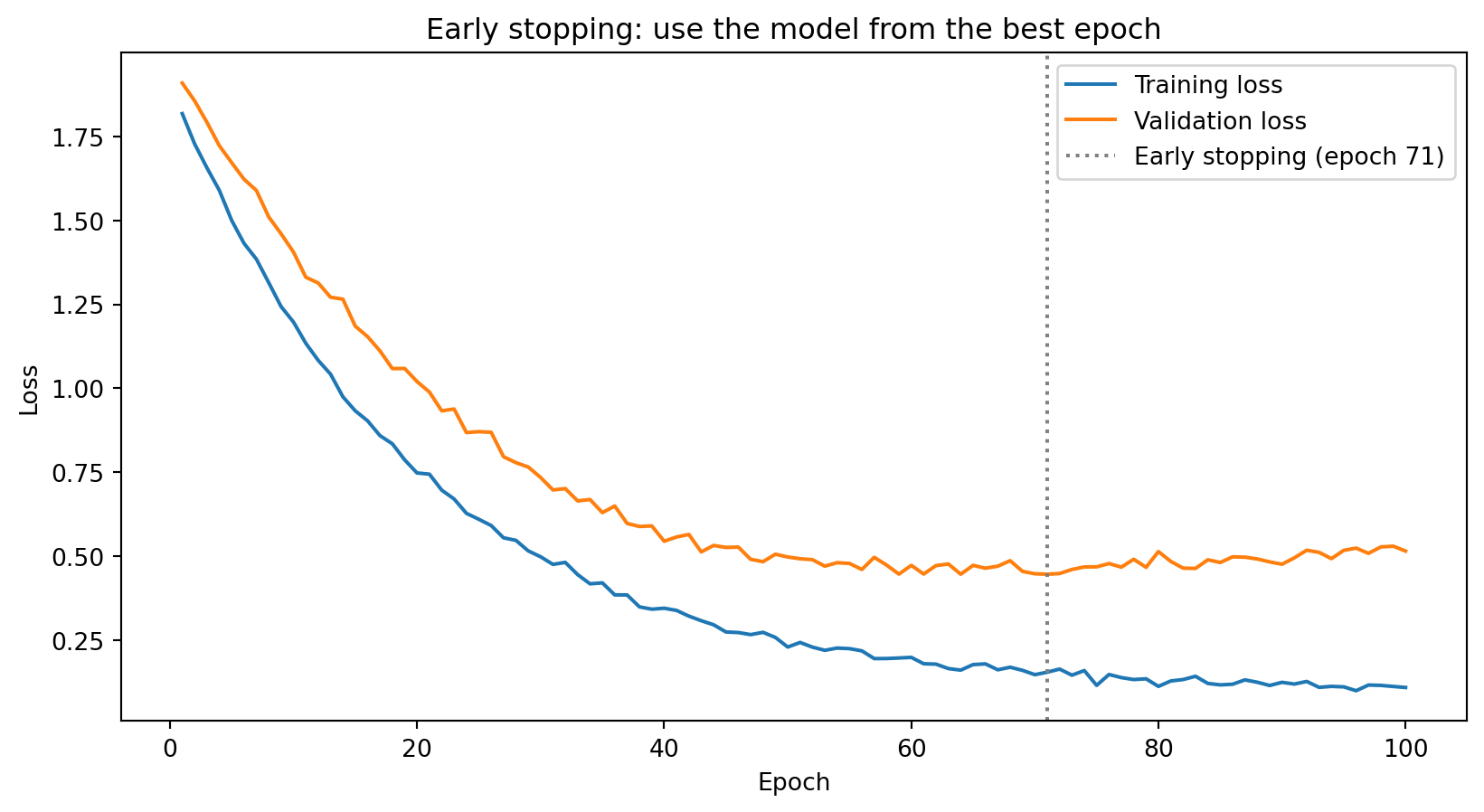
Early stopping acts as implicit regularization: by limiting the number of gradient descent steps, we prevent the model from fully fitting the training noise. It’s analogous to how reducing the number of boosting rounds controls overfitting in XGBoost.

Dropout

Dropout (Srivastava et al., 2014): at each mini-batch, randomly set a fraction of neurons to zero.

Each neuron is turned off independently with probability \(p\) (typically 0.2 to 0.5)
Surviving neurons must learn to predict without relying on any single neuron

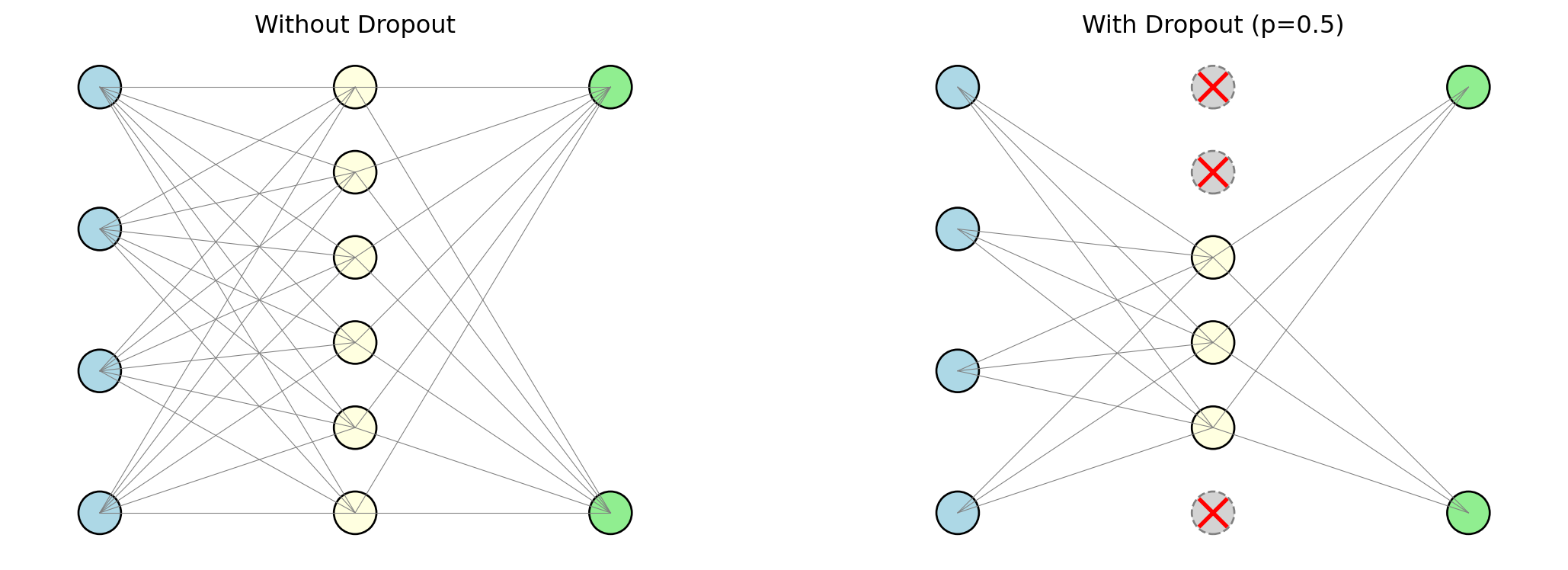
Ensemble interpretation: each mini-batch trains a slightly different sub-network → the final model is an average over all of them (like Random Forests averaging trees)
At test time: dropout is turned off, all neurons are used, weights are scaled accordingly

Weight Decay (L2 Regularization)

Same L2 penalty as Ridge regression, applied to neural network weights:

\[\mathcal{L}_{\text{total}} = \mathcal{L}_{\text{data}} + \lambda \sum_{\ell} \|\mathbf{W}^{(\ell)}\|_2^2\]

The gradient update now includes a term that pulls weights toward zero:

\[w_{t+1} = w_t - \eta \frac{\partial \mathcal{L}_{\text{data}}}{\partial w_t} - \underbrace{\eta \lambda w_t}_{\text{decay}}\]

The \(-\eta \lambda w_t\) term shrinks each weight at every step → called weight decay
Encourages small, diffuse weights rather than a few strong connections
Same logic as Ridge: constrain parameters to prevent fitting noise

Deep vs. Wide Networks

Two ways to add capacity to a network:

Wider: More neurons per layer (e.g., one hidden layer with 1,000 neurons)

Deeper: More layers with fewer neurons each (e.g., five hidden layers with 64 neurons each)

The universal approximation theorem says one wide layer is sufficient. In practice, deeper is often better:

Hierarchical representations: early layers detect simple patterns, later layers combine them (edges → shapes → objects)
Parameter-efficient: some functions need exponentially many neurons in one layer but only a few layers deep
Harder to train: vanishing gradients, more hyperparameters, longer training

For tabular financial data: 2–4 hidden layers usually suffice. 50+ layers are for images, text, and structured data.

Batch Normalization and Layer Normalization

As preceding layers change during training, the distribution of each layer’s inputs shifts (internal covariate shift). Normalization techniques fix this.

Batch Normalization (Ioffe & Szegedy, 2015) — normalize across the mini-batch:

\[\hat{z} = \frac{z - \mu_{\text{batch}}}{\sigma_{\text{batch}}}\]

The network learns two extra parameters per neuron (\(\gamma\), \(\beta\)) to scale and shift if needed

Layer Normalization (Ba, Lei & Hinton, 2016) — normalize across features within each observation:

Works better for small batch sizes
Standard for transformer architectures

Both stabilize training, allow higher learning rates, and act as mild regularizers.

Summary of Regularization Techniques

Technique	What it does	Analogy
Early stopping	Stop before the model overfits	Limiting boosting rounds in XGBoost
Dropout	Randomly disable neurons during training	Ensemble averaging (like Random Forests)
Weight decay	Penalize large weights (L2 penalty)	Ridge regression’s \(\lambda \\|\boldsymbol{\beta}\\|_2^2\)
Batch / Layer norm	Normalize intermediate values	Standardizing features before regression

In practice, these techniques are often combined. A typical setup: ReLU activation + Adam optimizer + dropout (0.2–0.5) + early stopping + some weight decay.

Part VI: Demo — Neural Networks in PyTorch

PyTorch: The Standard Framework

PyTorch is the most widely used deep learning framework in research and increasingly in industry. It handles all the backpropagation, gradient computation, and optimization automatically — you define the architecture and the training loop.

We’ll build a simple classifier for the same synthetic data we used with Random Forests and XGBoost.

import numpy as np
import torch
import torch.nn as nn
from sklearn.datasets import make_classification
from sklearn.model_selection import train_test_split
from sklearn.preprocessing import StandardScaler

# Generate data
X, y = make_classification(
    n_samples=1000, n_features=10, n_informative=5,
    random_state=42
)

# Split into train, validation, and test
X_temp, X_test, y_temp, y_test = train_test_split(
    X, y, test_size=0.2, random_state=42
)
X_train, X_val, y_train, y_val = train_test_split(
    X_temp, y_temp, test_size=0.2, random_state=42
)

# Standardize features (neural networks are sensitive to feature scales)
scaler = StandardScaler()
X_train = scaler.fit_transform(X_train)
X_val = scaler.transform(X_val)
X_test = scaler.transform(X_test)

# Convert to PyTorch tensors
X_train_t = torch.tensor(X_train, dtype=torch.float32)
y_train_t = torch.tensor(y_train, dtype=torch.float32).unsqueeze(1)
X_val_t = torch.tensor(X_val, dtype=torch.float32)
y_val_t = torch.tensor(y_val, dtype=torch.float32).unsqueeze(1)
X_test_t = torch.tensor(X_test, dtype=torch.float32)
y_test_t = torch.tensor(y_test, dtype=torch.float32).unsqueeze(1)

print(f"Training set:   {X_train_t.shape[0]} observations")
print(f"Validation set: {X_val_t.shape[0]} observations")
print(f"Test set:       {X_test_t.shape[0]} observations")

Training set:   640 observations
Validation set: 160 observations
Test set:       200 observations

Building the Model

# Build a feed-forward neural network
model = nn.Sequential(
    nn.Linear(10, 64),   # hidden layer 1: 64 neurons
    nn.ReLU(),
    nn.Linear(64, 32),   # hidden layer 2: 32 neurons
    nn.ReLU(),
    nn.Linear(32, 1),    # output layer: 1 neuron
    nn.Sigmoid()          # sigmoid for binary classification
)

# Choose optimizer and loss function
optimizer = torch.optim.Adam(model.parameters(), lr=0.001)
loss_fn = nn.BCELoss()  # binary cross-entropy

print(model)
print(f"\nTotal parameters: {sum(p.numel() for p in model.parameters()):,}")

Sequential(
  (0): Linear(in_features=10, out_features=64, bias=True)
  (1): ReLU()
  (2): Linear(in_features=64, out_features=32, bias=True)
  (3): ReLU()
  (4): Linear(in_features=32, out_features=1, bias=True)
  (5): Sigmoid()
)

Total parameters: 2,817

Each Linear layer is a fully-connected layer (every neuron connects to every neuron in the previous layer). ReLU activations introduce nonlinearity between layers.

Training the Model

from torch.utils.data import TensorDataset, DataLoader

# Create data loader for mini-batching
train_loader = DataLoader(TensorDataset(X_train_t, y_train_t), batch_size=32, shuffle=True)

# Training loop
train_losses = []
val_losses = []

torch.manual_seed(42)

for epoch in range(50):
    # Training phase
    for X_batch, y_batch in train_loader:
        optimizer.zero_grad()           # reset gradients
        y_pred = model(X_batch)         # forward pass
        loss = loss_fn(y_pred, y_batch) # compute loss
        loss.backward()                 # backpropagation
        optimizer.step()                # update weights

    # Record losses (no gradients needed for evaluation)
    with torch.no_grad():
        train_losses.append(loss_fn(model(X_train_t), y_train_t).item())
        val_losses.append(loss_fn(model(X_val_t), y_val_t).item())

print(f"Final training loss: {train_losses[-1]:.4f}")
print(f"Final validation loss: {val_losses[-1]:.4f}")

Final training loss: 0.0821
Final validation loss: 0.1823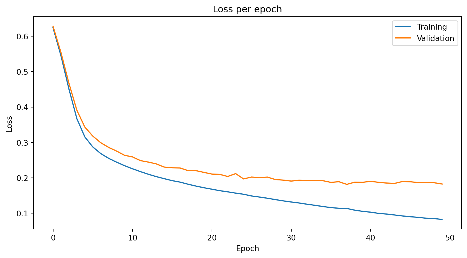

Training loss is consistently below validation loss — the model fits the training data better than unseen data, as expected. The gap is small here, meaning the model generalizes reasonably well.

Evaluating on the Test Set

# Evaluate on the held-out test set
with torch.no_grad():
    test_pred = model(X_test_t)
    test_accuracy = ((test_pred > 0.5) == y_test_t).float().mean().item()

print(f"Test accuracy: {test_accuracy:.3f}")

Test accuracy: 0.950

# Compare with Random Forest and XGBoost on the same data
from sklearn.ensemble import RandomForestClassifier
from xgboost import XGBClassifier

rf = RandomForestClassifier(n_estimators=200, random_state=42)
rf.fit(X_train, y_train)

xgb = XGBClassifier(n_estimators=200, learning_rate=0.1, max_depth=3, random_state=42)
xgb.fit(X_train, y_train)

print(f"\nModel comparison on test set:")
print(f"Neural Network: {test_accuracy:.3f}")
print(f"Random Forest:  {rf.score(X_test, y_test):.3f}")
print(f"XGBoost:        {xgb.score(X_test, y_test):.3f}")


Model comparison on test set:
Neural Network: 0.950
Random Forest:  0.950
XGBoost:        0.945

On small tabular datasets like this, neural networks typically perform comparably to tree-based methods — sometimes slightly better, sometimes slightly worse. The real advantage of neural networks emerges with large datasets and non-tabular data (images, text, sequences).

Neural Networks in Finance: Where They Shine

Application	Why neural networks?
High-frequency trading	Large datasets, complex nonlinear patterns in order flow
Factor models	Gu, Kelly & Xiu (2020): NNs outperform linear/tree models for stock return prediction — but need large panels
Alternative data	Images, news, earnings calls, social media require specialized architectures (CNNs, transformers)
Risk management	Estimating loss distributions, stress testing, credit risk

Where tree-based models still win: small-to-medium tabular datasets (most day-to-day finance). XGBoost/RF are competitive, faster to train, easier to tune, and interpretable.

Neural Network Hyperparameters: A Summary

Hyperparameter	What it controls	Typical choices
Number of layers	Network depth	2–4 for tabular data; dozens for images/text
Neurons per layer	Network width	32, 64, 128, 256
Activation function	Nonlinearity type	ReLU (hidden), sigmoid/softmax (output)
Learning rate	Step size in gradient descent	0.001 (Adam), 0.01 (SGD)
Batch size	Observations per gradient update	32–256
Epochs	Passes through training data	Until validation loss stops improving
Dropout rate	Fraction of neurons dropped	0.2–0.5
Weight decay	L2 penalty strength	\(10^{-4}\) to \(10^{-2}\)
Optimizer	Gradient descent variant	Adam (default), SGD with momentum

Start with a simple architecture (2 hidden layers, 64 neurons each, ReLU, Adam, dropout 0.3) and adjust based on validation performance.

Tuning Hyperparameters: A Practical Guide

Start simple. 2 hidden layers, 64 neurons each. Can the model overfit the training data? If not, fix the architecture or learning rate first.
Get the learning rate right. Loss barely moves → increase. Loss explodes → decrease. Try \(10^{-2}, 10^{-3}, 10^{-4}\).
Regularize. Once you can overfit, add dropout (0.2–0.3), early stopping, and/or weight decay to close the train–val gap.
Scale up if needed. Val loss high and close to train loss → underfitting (go wider/deeper). Big gap → overfitting (more regularization or smaller network).

Common Pitfalls

Tuning too many things at once. Change one hyperparameter at a time — otherwise you won’t know what helped.
Not standardizing inputs. Feature scales matter. A feature in billions and one in decimals → gradients dominated by the large one. Always standardize first.
No early stopping. The model will memorize. Monitor validation loss.
Too deep too soon. For tabular data, 2–4 layers usually suffice. Start shallow.
Ignoring the baseline. Always compare against logistic regression or Random Forest. If the NN doesn’t beat it, the complexity isn’t worth it.
Forgetting model.eval(). Dropout and batch norm behave differently during training vs. evaluation. Always switch modes.

Part VII: Beyond Feed-Forward Networks

Beyond Feed-Forward: Specialized Architectures

The feed-forward networks we’ve been building treat each input as a flat vector of numbers — no notion of spatial structure, no notion of order, no notion of time. That’s fine for tabular data (rows of features), but many real-world problems have richer structure:

Images have spatial layout — nearby pixels are related, and patterns like edges recur across the image
Sequences have order — the meaning of a word depends on the words before and after it
High-dimensional data may have a low-dimensional structure hiding underneath

Each of the architectures in this section was designed to exploit a specific kind of structure. We won’t go deep into the math — the formulas get heavy — but you should understand what problem each one solves and why it was a breakthrough.

Convolutional Neural Networks (CNNs)

CNNs are the standard architecture for image data. They exploit a basic property of images: nearby pixels contain similar information — the same “edge detector” is useful everywhere in the image.

A feed-forward network would assign one weight per pixel and connect every pixel to every neuron. For a 256×256 image, that’s 65 million weights in the first layer alone — most of them redundant.
Instead, a CNN uses weight sharing: a small filter (say, 3×3 pixels) slides across the entire image, applying the same weights at every position. This dramatically reduces the parameter count and prevents overfitting.
The filter slides over \(n \times n\) blocks of pixels, producing a feature map that says “how strongly did this pattern appear here?” Stack many filters to detect many patterns, then repeat — building up from simple edges to complex shapes.
Because the inputs are 2D (or 3D with colour channels), the weight matrices become higher-dimensional arrays — tensors. The math generalizes from matrix multiplication to tensor operations, which gets ugly fast. The ideas are the same; the notation just has more indices.

CNNs: The LeNet-5 Architecture

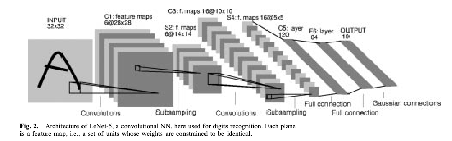
LeCun, Bottou, Bengio & Haffner (1998), Figure 2

LeNet-5 was designed to read handwritten cheques for banks — one of the first commercially deployed neural networks. Input image → convolutional filters → pooling (downsampling) → more filters → fully connected layer → output. The same architectural principles now power image recognition, medical imaging, and satellite analysis.

Autoencoders

The problem: You have high-dimensional data (hundreds of features) but suspect that the variation is really driven by a smaller number of underlying factors. How do you find that low-dimensional structure?

A classical approach is Principal Component Analysis (PCA). PCA finds the directions of maximum variance in the data and projects onto them — compressing, say, 100 features into 5 “principal components” that capture most of the variation. It works well, but it can only find linear combinations of the original features. If the true low-dimensional structure is nonlinear (curved, folded, or otherwise complex), PCA will miss it.

The idea: Train a neural network to reconstruct its own input — but force the data through a narrow bottleneck in the middle. If the network can reconstruct the input well despite the bottleneck, the bottleneck must have learned a compressed representation that captures the essential structure. Because the encoder and decoder are neural networks, this compression can be nonlinear — it’s PCA without the linearity constraint.

Autoencoders: The Architecture

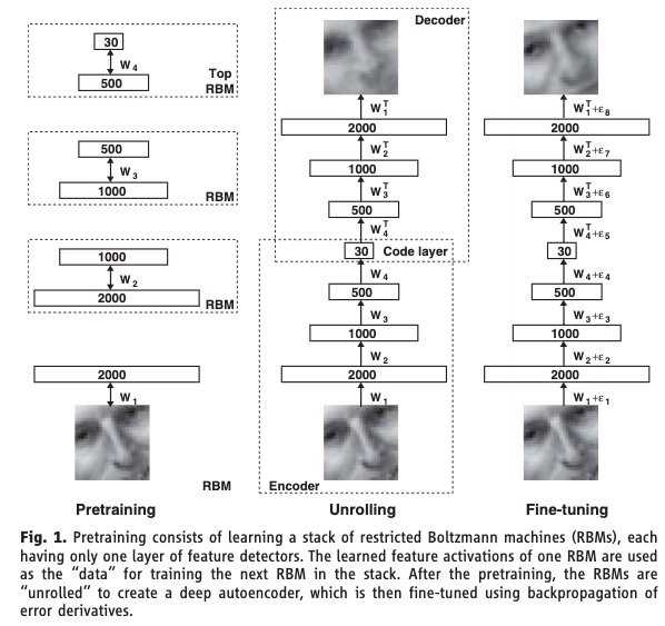
Autoencoders: How They Work

The encoder maps the high-dimensional input down to a low-dimensional latent representation (the bottleneck) — say, compressing 100 features into 5
The decoder maps the latent representation back up to the original dimension
The loss function is reconstruction error: how well does the output match the input?
The network is never given labels — this is unsupervised learning

Hinton & Salakhutdinov (2006) showed that deep autoencoders dramatically outperform PCA for dimensionality reduction. This Science paper was a catalyst for the modern deep learning resurgence. A later variant, the Variational Autoencoder (VAE) by Kingma & Welling (2014), adds a probabilistic twist that allows the decoder to generate new data by sampling from the bottleneck.

Recurrent Neural Networks (RNNs)

The problem: Feed-forward networks treat each input independently. But many financial signals are sequential — the meaning of today’s return depends on what happened yesterday, last week, and last month. An earnings call transcript is a sequence of words where order matters. A limit order book evolves through time.

The idea: Give the network a memory. At each time step, the network receives the current input and a summary of everything it has seen so far.

How it works:

At each step \(t\), the network takes in the current input \(x_t\) and the previous hidden state \(h_{t-1}\)
It produces a new hidden state \(h_t\) that encodes everything seen up to time \(t\)
The output prediction is computed from \(h_t\)
The same weights are reused at every time step — the network learns a single “update rule” that applies across the entire sequence

The seminal paper: Rumelhart, Hinton & Williams (1986). The backpropagation framework from PDP laid the foundation for training networks with recurrent connections — hidden states that feed back into themselves across time steps.

The trouble is that for long sequences, the hidden state has to carry information through many steps. In practice, the gradient signal degrades over long chains — the vanishing gradient problem again. By the time the network reaches step 100, it has effectively forgotten what happened at step 1.

Long Short-Term Memory (LSTM)

The problem with vanilla RNNs: they can’t remember things for more than a handful of time steps. For financial applications — where a quarterly earnings surprise might affect prices for months — this is a serious limitation.

The fix: add a separate memory channel (the “cell state”) with learned gates that control what to remember and what to forget.

Think of the cell state as a conveyor belt running above the network. At each time step, three gates decide:

Forget gate: What old information to discard — “that earnings call was two quarters ago, it’s no longer relevant”
Input gate: What new information to store — “this surprise Fed announcement is important, write it to memory”
Output gate: What part of the memory to use for the current prediction — “for today’s forecast, the recent volatility regime matters most”

Each gate is a small neural network that learns when to open and close from the data. The cell state can carry information forward across many time steps without degradation, because the forget gate can stay close to 1 (meaning “keep everything”) when the information is still relevant.

The seminal paper: Hochreiter & Schmidhuber (1997). LSTMs became the dominant architecture for sequence modelling for nearly two decades, until transformers overtook them.

Transformers

The problem with RNNs/LSTMs: They process sequences one step at a time, left to right. Step 50 has to wait for steps 1–49 to finish — this is slow, and it means the model can’t be parallelized across time steps. Worse, even LSTMs struggle when related pieces of information are far apart in the sequence. Consider: “The executive who the board hired last quarter after a lengthy search resigned.” — subject and verb are nine words apart, and the RNN has to carry the subject through all the intervening words.

The idea: Throw away recurrence entirely. Instead, let every element in the sequence look at every other element directly, all at once. This mechanism is called self-attention.

How self-attention works:

Each element in the sequence (a word, a time step) gets projected into three roles:

Query: “What am I looking for?”
Key: “What do I have to offer?”
Value: “Here is my actual content.”

For every pair of elements, the model computes a relevance score (how much does element A care about element B?) by comparing A’s query to B’s key. These scores become attention weights — and each element’s new representation is a weighted average of all the values in the sequence.

The critical advantage: all pairwise scores are computed simultaneously as a single matrix multiplication. This means the entire sequence is processed in parallel on a GPU, regardless of length. And any two elements can interact directly — no information needs to “survive” through intermediate steps.

The seminal paper: Vaswani, Shazeer, Parmar, Uszkoreit, Jones, Gomez, Kaiser & Polosukhin (2017). “Attention Is All You Need” — one of the most cited papers in machine learning history. Transformers are the architecture behind GPT, Claude, and every modern large language model.

Generative Adversarial Networks (GANs)

The problem: Every model we’ve built so far is discriminative — it maps inputs to outputs (\(\mathbf{x} \to y\)). But what if you need to generate new data that looks realistic? Synthetic financial data for stress testing, privacy-preserving data sharing, augmenting small training sets.

The idea: Train two networks against each other in a game. One tries to generate realistic fakes; the other tries to spot them. The competition drives both to improve.

How it works:

The Generator takes random noise as input and produces a synthetic data point — a fake stock return series, a fabricated earnings report, a simulated portfolio path
The Discriminator takes a data point (either real from the training set or fake from the generator) and tries to classify it as real or fake
They train in alternation: the discriminator gets better at detecting fakes, which forces the generator to produce more convincing fakes, which forces the discriminator to get even better, and so on
At convergence (in theory), the generator produces data so realistic that the discriminator can’t tell the difference and guesses randomly

In practice, GAN training is notoriously unstable — the two networks can oscillate rather than converge, and the generator can collapse to producing only a few types of output. Despite this, GANs have produced remarkable results in image generation and are increasingly used in finance.

The seminal paper: Goodfellow, Pouget-Abadie, Mirza, Xu, Warde-Farley, Ozair, Courville & Bengio (2014).

Diffusion Models

The problem with GANs: They’re powerful but notoriously hard to train. The generator and discriminator can oscillate instead of converging, and the generator often suffers from mode collapse — it learns to produce only a narrow range of outputs rather than the full diversity of the training data. Researchers wanted a generative approach that was more stable and produced higher-quality, more diverse outputs.

The idea: Instead of learning to generate data in one shot (like a GAN), learn to reverse a gradual noising process. Start with real data and slowly add random noise over many steps until it becomes pure static. Then train a neural network to reverse each step — to take slightly noisy data and make it slightly less noisy. To generate new data, start from pure noise and apply the learned denoising steps repeatedly until a clean sample emerges.

How it works:

Forward process (fixed): Take a training example \(\mathbf{x}_0\) and add a small amount of Gaussian noise at each step \(t = 1, 2, \ldots, T\). After enough steps, \(\mathbf{x}_T\) is indistinguishable from pure random noise. This process requires no learning — it’s just a schedule of noise additions.
Reverse process (learned): Train a neural network \(\epsilon_\theta(\mathbf{x}_t, t)\) to predict the noise that was added at each step. Given a noisy \(\mathbf{x}_t\) and the step number \(t\), the network learns to estimate what noise to subtract to recover \(\mathbf{x}_{t-1}\).
Generation: Sample pure noise \(\mathbf{x}_T \sim \mathcal{N}(0, I)\), then apply the learned denoising network \(T\) times to walk back to a clean sample \(\mathbf{x}_0\).

The key advantage over GANs: there is no adversarial training, so no mode collapse and no training instability. The trade-off is that generation is slower — you need many denoising steps rather than a single forward pass. Diffusion models are the architecture behind DALL-E, Stable Diffusion, and modern image/video generation systems, and have largely displaced GANs as the dominant generative approach.

The seminal paper: Ho, Jain & Abbeel (2020). “Denoising Diffusion Probabilistic Models.”

Architecture Summary

Architecture	Problem it solves	How	Seminal paper
CNN	Spatial structure (images)	Local filters + weight sharing	LeCun et al. (1998)
Autoencoder	Dimensionality reduction	Compress through bottleneck, reconstruct	Hinton & Salakhutdinov (2006)
RNN	Sequential data	Hidden state carries memory through time	Rumelhart, Hinton & Williams (1986)
LSTM	Long-range dependencies in sequences	Cell state with learned gates	Hochreiter & Schmidhuber (1997)
Transformer	Long-range dependencies + parallelism	Self-attention over entire sequence at once	Vaswani et al. (2017)
GAN	Generating synthetic data	Two networks compete (generator vs. discriminator)	Goodfellow et al. (2014)
Diffusion	Stable, high-quality generation	Learn to reverse a gradual noising process	Ho, Jain & Abbeel (2020)

Each of these uses the same building blocks from earlier in this lecture — neurons, layers, activations, backpropagation, gradient descent. The difference is how the layers are connected and what structure in the data they’re designed to exploit.

My Research: Finance-Informed Neural Networks

Every model we’ve seen today uses data to train: we have \((x_i, y_i)\) pairs and minimize a loss like MSE. But what if we don’t have data — we have an equation we know the solution must satisfy?

Many problems in finance boil down to: find a function \(f\) such that some condition like \(f(x) = 0\) holds
We know from theory what the equation is, but we can’t solve it by hand — especially when the problem is high-dimensional
The idea: let \(f_\theta\) be a neural network, and use the equation itself as the loss function. If the equation says \(f(x) = 0\), then \(\mathcal{L} = \sum_i f_\theta(x_i)^2\) — this is zero when \(f_\theta\) satisfies the equation, positive when it doesn’t. Gradient descent does the rest.

This idea originated in physics (Raissi, Perdikaris & Karniadakis, 2019), where it’s called Physics-Informed Neural Networks (PINNs). My dissertation applied it to finance — Finance-Informed Neural Networks (FINNs) — in two settings.

FINNs Application 1: Macroeconomic Policy (Chapters 1 & 2)

Model 60 overlapping generations of households (ages 20–79)–3 types: 0- ,low-, high-LTI–each choosing how much to consume vs. save. A household of age \(i\) maximizes lifetime utility — the discounted sum of utility from consumption over its remaining life:

\[\max \quad \mathbb{E}_t \sum_{s=0}^{59} \beta^s \; u(c_{i,t+i})\]

subject to a budget constraint each period:

\[c_{i,t} + k_{i+1,t+1} = (1-\tau_t)\,w_t\,\ell_i + (1 + r_t)\,k_{i,t} - a_{i,t}\]

where \(c_{i,t}\) is consumption, \(k_{i+1,t+1}\) is savings carried into next period, \(w_t\,\ell_i\) is after-tax labour income, \(r_t\) is the return on savings, and \(a_{i,t}\) is the student loan payment. This budget constraint is what links all the households together — everyone’s savings become the economy’s capital, which determines next period’s wages and returns for everyone else.

When you solve this optimization (take the first-order condition), you get a condition that must hold at every age: the marginal benefit of consuming one more dollar today must equal the expected marginal benefit of saving that dollar and consuming it tomorrow:

\[u'(c_{i,t}) = \beta \; \mathbb{E}_t\!\left[u'(c_{i+1,t+1}) \cdot (1 + r_{t+1})\right]\]

where \(u'(\cdot)\) is marginal utility, \(\beta\) is the discount factor (patience), and \(r_{t+1}\) is the return on savings. In words: if this condition is violated, the household can do better by shifting consumption between today and tomorrow.

That’s 59 \(\times\) 3 of these conditions (one per age per type) that must all hold simultaneously. The state space — tracking everyone’s wealth — is 178-dimensional. Traditional methods that use grids are hopeless here: a grid with just 10 points per dimension would have \(10^{178}\) grid points.

Instead, a neural network \(f_\theta\) learns the optimal saving decision for all 60 age groups at once, trained by penalizing violations of these optimality conditions. To avoid grids entirely, I use the neural network’s own policy to simulate the economy forward in time — generating a time series of states the economy actually visits — and evaluate the optimality conditions only at those points. No grid, no curse of dimensionality.

FINNs Application 2: Pricing Interest Rate Derivatives (Chapter 3)

A caplet is an option on a future interest rate — it pays off if the rate exceeds a strike \(L_E\). From RSM332, the price of any derivative is the expected discounted payoff under no-arbitrage:

\[V(t) = \mathbb{E}\!\left[\exp\!\left(-\int_t^T r(s)\,ds\right) \cdot \text{payoff at } T\right]\]

where \(r(s)\) is the short-term interest rate along the path. The standard approach is Monte Carlo simulation: simulate thousands of random interest rate paths, compute the payoff on each, discount back, and average. This is slow — seconds per contract — and you need to re-simulate for every change in contract terms.

Instead, there is an equivalent way to express exactly the same price, not as an expectation over random paths, but as a deterministic equation that the price function \(V\) must satisfy:

\[-\frac{\partial V}{\partial \tau} + \mu' \nabla_f V + \frac{1}{2} \sum_{n=1}^{N} \sigma_n' \nabla_f^2 V \; \sigma_n - r \cdot V = 0\]

where \(\tau\) is time to maturity, \(f\) is the current forward rate curve, and \(\mu, \sigma\) come from the term structure model. You don’t need to understand every symbol here — the point is that this is an equation the price must satisfy, and it involves derivatives of \(V\) with respect to its inputs.

A neural network \(V_\theta\) approximates the price. The loss function squares the left-hand side of that equation: if \(V_\theta\) satisfies the equation, the loss is zero. Backpropagation — the same machinery used to train any neural network — computes all the partial derivatives of \(V_\theta\) that appear in the equation. No random simulation at all — the network learns the price by satisfying the equation directly.

The result: once trained, the network prices any contract instantly. Prices are 300,000–4,500,000\(\times\) faster than Monte Carlo simulation, with accuracy to 0.04 cents per dollar.

Summary and Preview

What We Learned Today

Deep learning = regression. A neural network is a choice of \(f_\theta\) in the same framework from Lecture 5. The loss functions, regularization, and evaluation methods all carry over.

The architecture. Neurons compute weighted sums plus nonlinear activations. Layers stack neurons together. Feed-forward networks chain layers sequentially. Activation functions (especially ReLU) are what make depth meaningful — without them, multiple layers collapse to a single linear transformation.

Universal approximation. A wide enough single-layer network can approximate any continuous function. But this is an existence theorem, not a practical recipe. Deep networks are more parameter-efficient and learn hierarchical representations.

Training. No closed-form solution — we use gradient descent. Backpropagation efficiently computes gradients by applying the chain rule backwards through the network. SGD with mini-batches makes training practical for large datasets. Adam is the default optimizer.

Regularization. Neural networks are massively overparameterized and prone to overfitting. Early stopping, dropout, weight decay, and batch normalization are the standard toolkit.

Specialized architectures. CNNs exploit spatial structure through local filters and weight sharing. Autoencoders learn compressed representations by reconstructing their own input through a bottleneck. RNNs and LSTMs handle sequential data by passing hidden states through time. Transformers replace recurrence with self-attention, processing entire sequences in parallel. GANs train two networks adversarially to generate synthetic data.

In practice. On tabular financial data, neural networks compete with but rarely dominate tree-based methods. Their real advantage is with large datasets and non-tabular data (images, text, sequences).

Next Lecture: Text and Natural Language Processing

Neural networks unlock a new kind of data for finance: text.

Earnings calls, news articles, analyst reports, SEC filings, social media — vast amounts of financially relevant information is locked in natural language.

Lecture 10: Text & Natural Language Processing

How to represent text as numbers
Bag-of-words, TF-IDF, and word embeddings
Sentiment analysis and topic modelling
Transformers and large language models

References

Ba, J. L., Kiros, J. R., & Hinton, G. E. (2016). Layer normalization. arXiv preprint arXiv:1607.06450.
Cybenko, G. (1989). Approximation by superpositions of a sigmoidal function. Mathematics of Control, Signals and Systems, 2(4), 303–314.
Goodfellow, I. J., Pouget-Abadie, J., Mirza, M., Xu, B., Warde-Farley, D., Ozair, S., Courville, A., & Bengio, Y. (2014). Generative adversarial nets. Advances in Neural Information Processing Systems, 27.
Gu, S., Kelly, B., & Xiu, D. (2020). Empirical asset pricing via machine learning. Review of Financial Studies, 33(5), 2223–2273.
Hastie, T., Tibshirani, R., & Friedman, J. (2009). The Elements of Statistical Learning (2nd ed.). Springer. Chapter 11.
Hinton, G. E. & Salakhutdinov, R. R. (2006). Reducing the dimensionality of data with neural networks. Science, 313(5786), 504–507.
Hochreiter, S. & Schmidhuber, J. (1997). Long short-term memory. Neural Computation, 9(8), 1735–1780.
Hornik, K. (1991). Approximation capabilities of multilayer feedforward networks. Neural Networks, 4(2), 251–257.
Ioffe, S. & Szegedy, C. (2015). Batch normalization: Accelerating deep network training by reducing internal covariate shift. Proceedings of ICML, 448–456.
Kingma, D. P. & Ba, J. (2015). Adam: A method for stochastic optimization. Proceedings of ICLR.
Kingma, D. P. & Welling, M. (2014). Auto-encoding variational bayes. Proceedings of ICLR.
LeCun, Y., Bottou, L., Bengio, Y., & Haffner, P. (1998). Gradient-based learning applied to document recognition. Proceedings of the IEEE, 86(11), 2278–2324.
Rumelhart, D. E., Hinton, G. E., & Williams, R. J. (1986). Learning representations by back-propagating errors. Nature, 323(6088), 533–536.
Srivastava, N., Hinton, G., Krizhevsky, A., Sutskever, I., & Salakhutdinov, R. (2014). Dropout: A simple way to prevent neural networks from overfitting. Journal of Machine Learning Research, 15, 1929–1958.
Vaswani, A., Shazeer, N., Parmar, N., Uszkoreit, J., Jones, L., Gomez, A. N., Kaiser, Ł., & Polosukhin, I. (2017). Attention is all you need. Advances in Neural Information Processing Systems, 30.