The notation \(P(y = 1 \,|\, \mathbf{x})\) reads “the probability that \(y = 1\)given\(\mathbf{x}\).” This is a conditional probability—the probability of default, given that we observe a particular set of feature values.
Here \(\mathbf{x} = (x_1, x_2, \ldots, x_p)'\) is a \(p\)-vector of features (attributes) for an observation, and \(\boldsymbol{\beta} = (\beta_1, \beta_2, \ldots, \beta_p)'\) is the corresponding \(p\)-vector of coefficients we need to learn.
The Linear Predictor
Let’s define \(z = \beta_0 + \boldsymbol{\beta}' \mathbf{x}\) as the linear predictor. Writing out the dot product:
The coefficient \(\beta_j\) tells us how a one-unit increase in \(x_j\) affects the log-odds:
If \(\beta_j > 0\): higher \(x_j\) increases the probability of \(y = 1\)
If \(\beta_j < 0\): higher \(x_j\) decreases the probability of \(y = 1\)
If \(\beta_j = 0\): \(x_j\) has no effect
We can also interpret coefficients as odds ratios: \(e^{\beta_j}\) is the multiplicative change in odds for a one-unit increase in \(x_j\). If \(\beta_j = 0.5\), then \(e^{0.5} \approx 1.65\): each one-unit increase multiplies the odds by 1.65 (a 65% increase).
Fitting Logistic Regression: The Loss Function
How do we find the best coefficients \(\beta_0, \boldsymbol{\beta}\)? Like any ML model, we define a loss function and minimize it.
For observation \(i\) with features \(\mathbf{x}_i\) and label \(y_i\), let \(\hat{p}_i = P(y_i = 1 \,|\, \mathbf{x}_i)\) be our predicted probability. Intuitively:
If \(y_i = 1\): we want \(\hat{p}_i\) close to 1 (predict high probability for actual positives)
If \(y_i = 0\): we want \(\hat{p}_i\) close to 0 (predict low probability for actual negatives)
The binary cross-entropy loss (also called log loss) captures this:
When \(y_i = 1\), the loss is \(-\ln(\hat{p}_i)\), which is small when \(\hat{p}_i\) is close to 1. When \(y_i = 0\), the loss is \(-\ln(1 - \hat{p}_i)\), which is small when \(\hat{p}_i\) is close to 0.
Comparing Loss Functions: Logistic vs. Linear Regression
Both linear and logistic regression fit into the same ML framework: define a loss function, then minimize it.
The choice of loss function depends on the problem: squared error makes sense for continuous outcomes, cross-entropy makes sense for probabilities.
Connection to statistics
In statistics, minimizing cross-entropy loss is equivalent to maximum likelihood estimation. Minimizing MSE is equivalent to maximum likelihood under the assumption that errors are normally distributed. Both approaches—ML and statistics—arrive at the same answer through different reasoning.
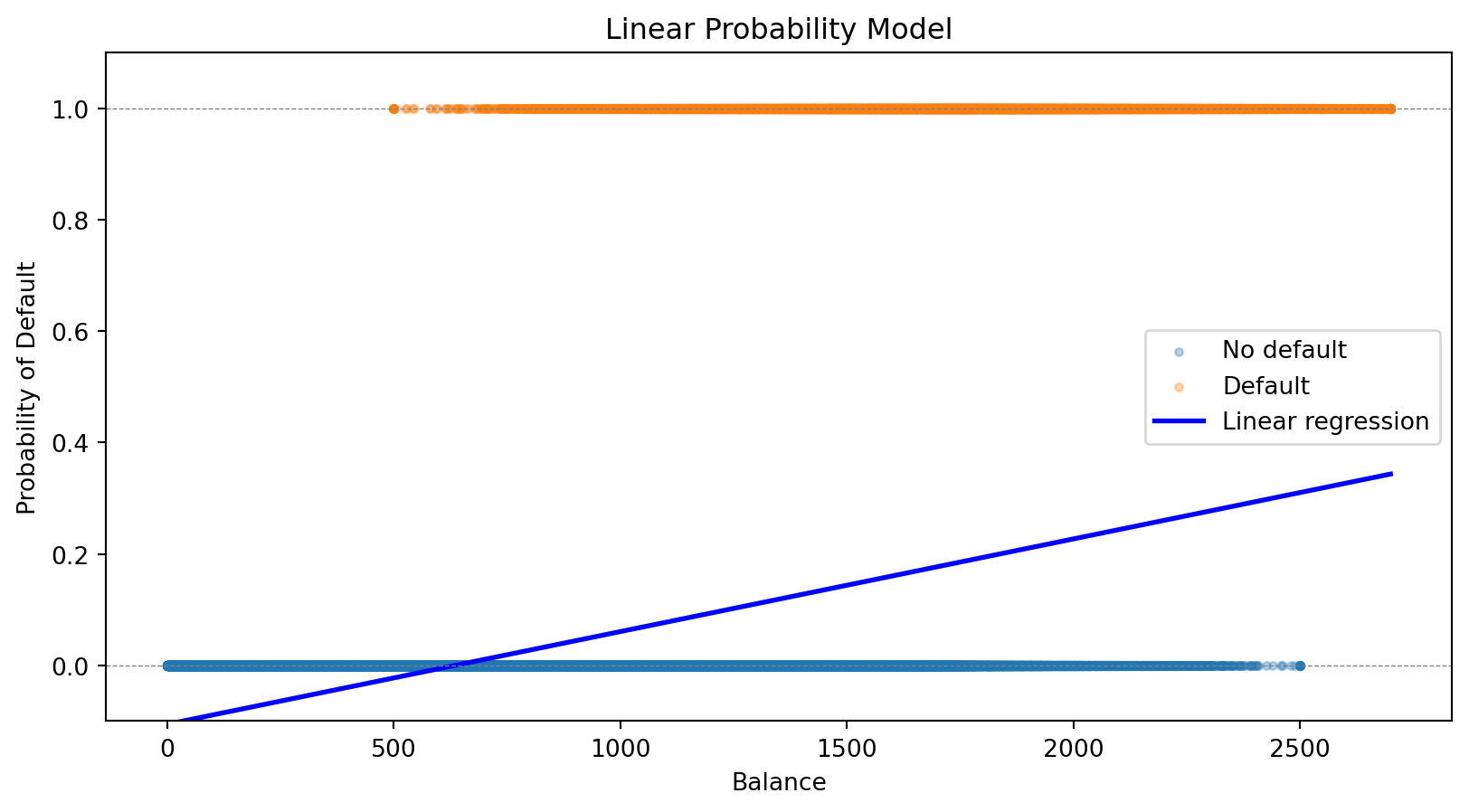
Logistic Regression for Credit Default
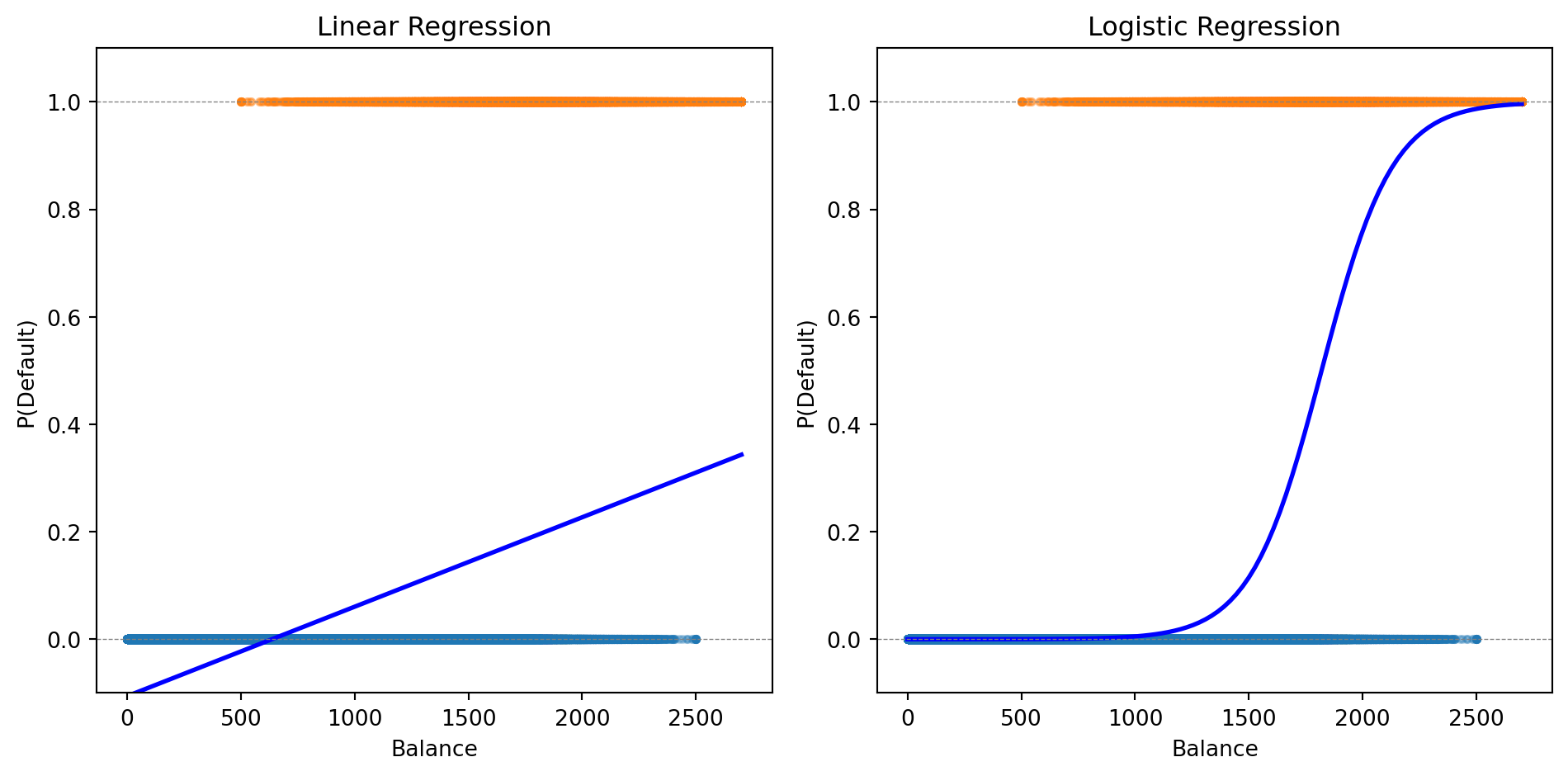
Let’s fit logistic regression to our credit default data:
from sklearn.linear_model import LogisticRegression# Fit logistic regressionlog_reg = LogisticRegression()log_reg.fit(X, y);# Predictionsprob_logistic = log_reg.predict_proba(balance_grid)[:, 1]print(f"Logistic Regression:")print(f" Intercept: {log_reg.intercept_[0]:.4f}")print(f" Coefficient on balance: {log_reg.coef_[0, 0]:.6f}")
Logistic Regression:
  Intercept: -11.6163
  Coefficient on balance: 0.006383
The logistic curve stays within [0, 1] and captures the S-shaped relationship between balance and default probability.
Making Predictions
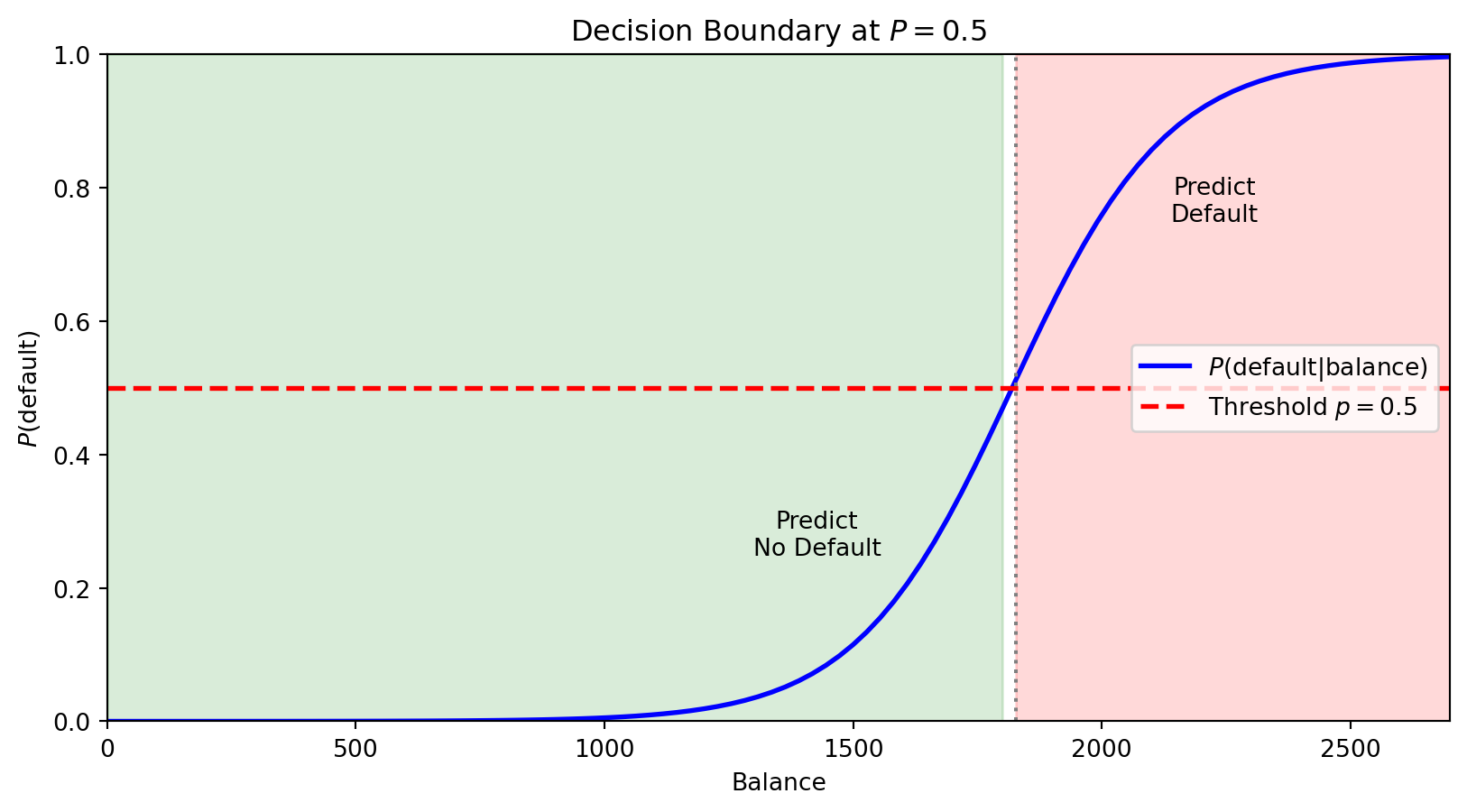
Logistic regression gives us a probability. To make a classification decision, we need a threshold (also called a cutoff).
The default rule: predict class 1 if \(P(y = 1 \,|\, \mathbf{x}) > 0.5\)
# Fit with both balance and incomeX_both = np.column_stack([balance, income])log_reg_both = LogisticRegression()log_reg_both.fit(X_both, default);print(f"Logistic Regression with Balance and Income:")print(f" Intercept: {log_reg_both.intercept_[0]:.4f}")print(f" Coefficient on balance: {log_reg_both.coef_[0, 0]:.6f}")print(f" Coefficient on income: {log_reg_both.coef_[0, 1]:.9f}")
Logistic Regression with Balance and Income:
  Intercept: -11.2532
  Coefficient on balance: 0.006383
  Coefficient on income: -0.000009279
The coefficient on income is tiny—income adds little predictive power beyond balance.
Multi-Class Logistic Regression
When we have \(K > 2\) classes, we can extend logistic regression using the softmax function.
For each class \(k\), we define a linear predictor:
The penalty \(\lambda \sum |\beta_j|\) shrinks coefficients toward zero and can set some exactly to zero (variable selection).
Benefits:
Prevents overfitting when \(p\) is large relative to \(n\)
Identifies which features matter most
Improves out-of-sample prediction
The regularization parameter \(\lambda\) is chosen by cross-validation.
from sklearn.linear_model import LogisticRegressionCV# Fit Lasso logistic regression with CVlog_reg_lasso = LogisticRegressionCV(penalty='l1', solver='saga', cv=5, max_iter=1000)log_reg_lasso.fit(X_both, default);print(f"Lasso Logistic Regression (λ chosen by CV):")print(f" Best C (inverse of λ): {log_reg_lasso.C_[0]:.4f}")print(f" Coefficient on balance: {log_reg_lasso.coef_[0, 0]:.6f}")print(f" Coefficient on income: {log_reg_lasso.coef_[0, 1]:.9f}")
Lasso Logistic Regression (λ chosen by CV):
  Best C (inverse of λ): 0.0001
  Coefficient on balance: 0.001064
  Coefficient on income: -0.000123556
Part III: Decision Boundaries
The Decision Boundary
Think of a classifier as drawing a line (or curve) through feature space that separates the classes. The decision boundary is this dividing line—observations on one side get predicted as Class 0, observations on the other side as Class 1.
For logistic regression with threshold 0.5, we predict Class 1 when \(P(y = 1 \,|\, \mathbf{x}) > 0.5\).
The boundary is where \(P(y = 1 \,|\, \mathbf{x}) = 0.5\) exactly—the point of maximum uncertainty.
The horizontal red line marks \(P = 0.5\). Where the probability curve crosses this threshold defines the decision boundary in feature space—observations with balance above this point are predicted to default.
With multiple features, the boundary is where \(\beta_0 + \beta_1 x_1 + \beta_2 x_2 + \cdots = 0\)—a linear equation in the features. This is why logistic regression is called a linear classifier: the decision boundary is a line (in 2D) or hyperplane (in higher dimensions).
What If Classes Aren’t Linearly Separable?
Sometimes a straight line can’t separate the classes well. If we know the structure of the problem, we can create curved boundaries by engineering the right features:
Include \(x_1^2\), \(x_2^2\), \(x_1 x_2\) as additional features
The model is still logistic regression (linear in these new features)
But the boundary is now curved in the original \((x_1, x_2)\) space
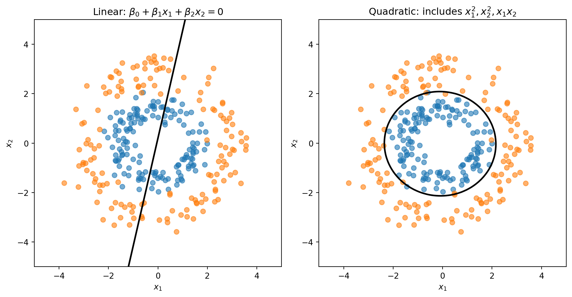
Linear vs. Quadratic Boundaries
Consider data where Class 0 forms an inner ring and Class 1 forms an outer ring. No straight line can separate these classes—we need a circular boundary.
A circle centered at the origin has equation \(x_1^2 + x_2^2 = r^2\). If we add squared terms as features, the decision boundary becomes:
This is a quadratic equation in \(x_1\) and \(x_2\)—it can represent circles, ellipses, or other curved shapes.
The linear model is forced to draw a straight line through the rings. The quadratic model can learn a circular boundary that actually separates the classes.
Another Approach: Classification as Supervised Clustering
Logistic regression directly models \(P(y = 1 \,|\, \mathbf{x})\). Linear Discriminant Analysis (LDA) takes the opposite approach — it models what each class looks like and uses Bayes’ theorem to classify.
The idea is the same as clustering (Lecture 4), except now we know the labels:
Assume each class \(k\) follows a multivariate normal: \(\mathbf{x} \mid y = k \;\sim\; \mathcal{N}(\boldsymbol{\mu}_k,\, \boldsymbol{\Sigma})\)
Estimate the class means \(\boldsymbol{\mu}_k\) and a shared covariance \(\boldsymbol{\Sigma}\) from training data
For a new observation, ask: which class’s distribution is it most likely to have come from?
Bayes’ theorem turns this into a scoring rule. The discriminant function for class \(k\) is:
where \(\pi_k = P(y = k)\) is the prior (just the fraction of training data in class \(k\)). Classify to whichever class has the highest \(\delta_k\). Because \(\delta_k\) is linear in \(\mathbf{x}\), the decision boundary is a line — just like logistic regression.
No optimization loop, no gradient descent — LDA computes its parameters in closed form. See the appendix for the full derivation.
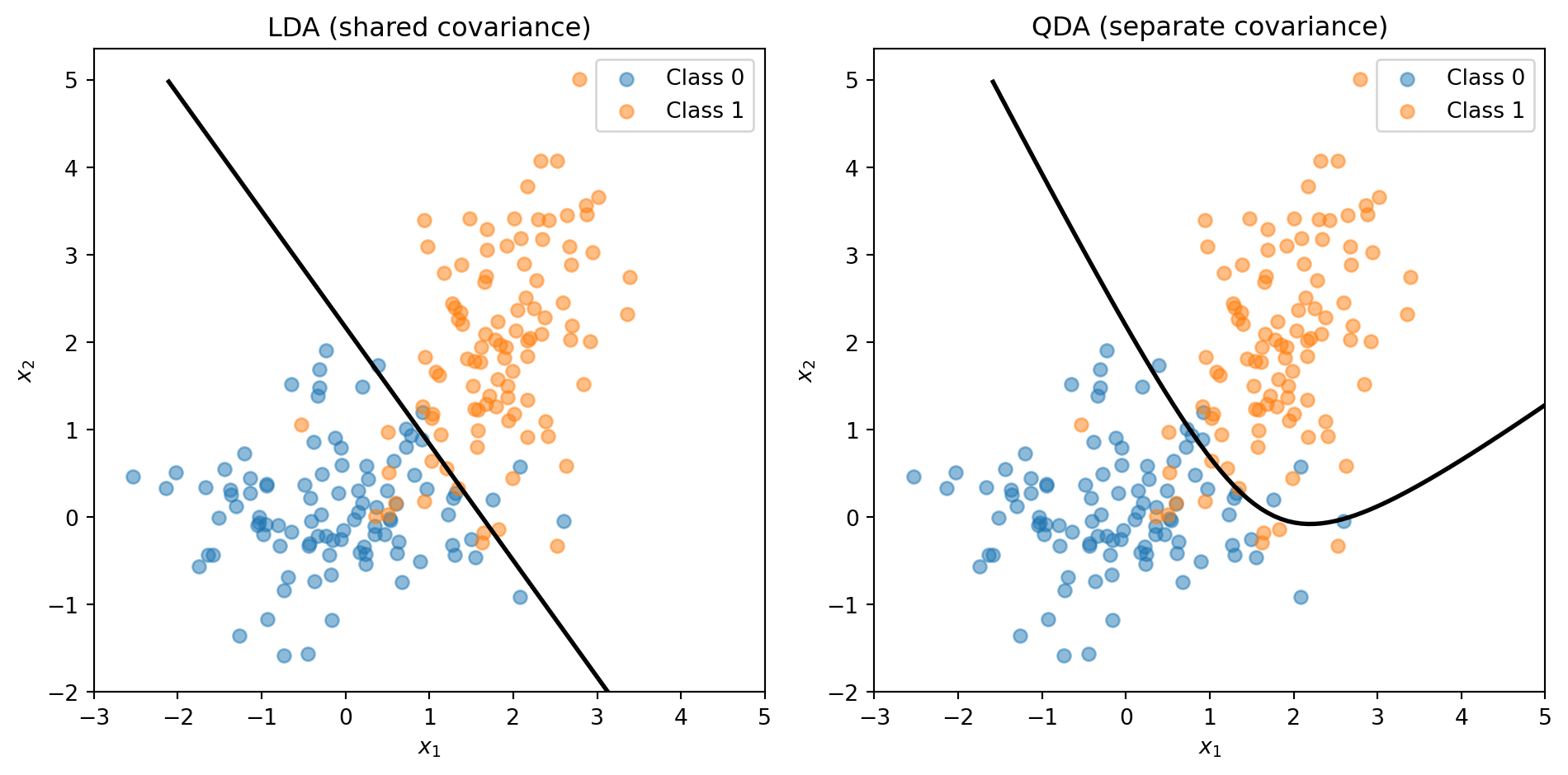
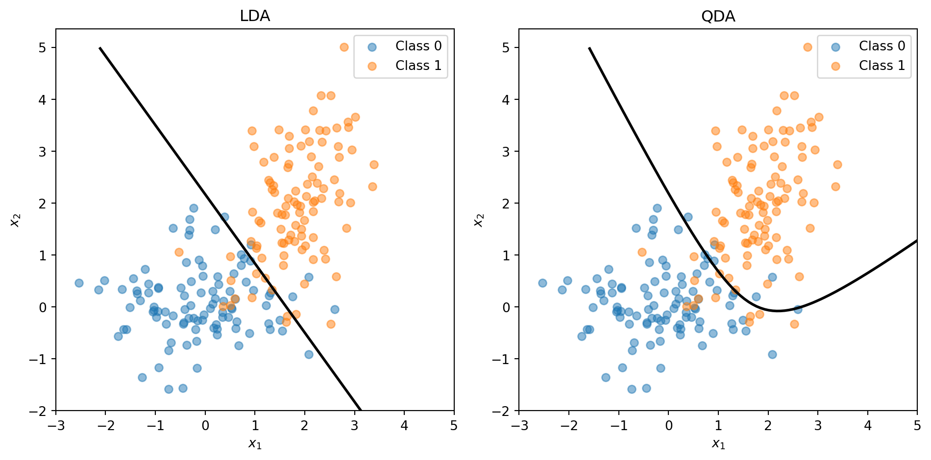
LDA vs. QDA: Shared or Separate Covariance?
LDA assumes all classes share the same covariance \(\boldsymbol{\Sigma}\) — same shape, different centres. Quadratic Discriminant Analysis (QDA) relaxes this: each class gets its own \(\boldsymbol{\Sigma}_k\).
Shared covariance → linear boundary (LDA)
Separate covariance → quadratic boundary (QDA)
The trade-off: LDA has fewer parameters (more stable, less overfitting); QDA is more flexible (captures curved boundaries). You’ll use both on the assignment. Full details in the appendix.
The Feature Engineering Problem
The ring example worked because we knew the right transformation: add \(x_1^2\) and \(x_2^2\). But that approach has a big limitation: we have to know which transformations to use.
With 2 features, adding squares and interactions is easy. With 50 features? There are 1,275 pairwise interactions and 50 squared terms—and we have no guarantee that quadratic terms are the right choice. Maybe the boundary depends on \(\log(x_3)\), or \(x_7 / x_{12}\), or something we’d never think to try.
We want methods that can learn nonlinear boundaries directly from the data, without us having to guess the right feature transformations in advance.
Parametric vs. Nonparametric Models
Parametric models (like logistic regression) assume the data follows a specific functional form. We estimate a fixed set of parameters (\(\beta_0, \beta_1, \ldots, \beta_p\)), and these parameters define the model completely.
Nonparametric models make fewer assumptions about the functional form. Instead, they let the data determine the structure of the decision boundary.
Parametric
Nonparametric
Structure
Fixed form (e.g., linear)
Flexible, data-driven
Parameters
Fixed number
Grows with data
Examples
Logistic regression, LDA
k-NN, Decision Trees
Risk
Bias if form is wrong
Overfitting with limited data
Both k-NN and decision trees are nonparametric—they don’t assume a linear (or any particular) decision boundary.
Part IV: k-Nearest Neighbors
The Intuition Behind k-NN
k-Nearest Neighbors (k-NN) is based on a simple idea: similar observations should have similar outcomes.
To classify a new observation:
Find the \(k\) training observations closest to it
Take a vote among those \(k\) neighbors
Assign the majority class
If you want to know if a new loan applicant will default, look at applicants in the training data who are most similar to them. If most of those similar applicants defaulted, predict default.
No training phase is needed—k-NN stores all the training data and does the work at prediction time. This is sometimes called a “lazy learner.”
Distance Recap (Lecture 4)
k-NN needs to measure how far apart two observations are. Same idea as clustering:
Standardize first. Features on different scales (income in dollars vs. DTI as a ratio) will make distance meaningless. Standardize each feature to mean 0, standard deviation 1.
Distance = norm of a difference. The \(L_2\) (Euclidean) norm is the default. Manhattan (\(L_1\)) is an alternative but Euclidean works well for most applications.
The k-NN Algorithm
Input: Training data \(\{(\mathbf{x}_1, y_1), \ldots, (\mathbf{x}_n, y_n)\}\), a new point \(\mathbf{x}\), and the number of neighbors \(k\).
Algorithm:
Compute the distance from \(\mathbf{x}\) to every training observation \(\mathbf{x}_i\)
Identify the \(k\) training observations with the smallest distances—call this set \(\mathcal{N}_k(\mathbf{x})\)
Assign the class that appears most frequently among the \(k\) neighbors:
The notation \(\unicode{x1D7D9}_{\{y_i = c\}}\) is the indicator function: it equals 1 if \(y_i = c\) and 0 otherwise. So we’re just counting votes.
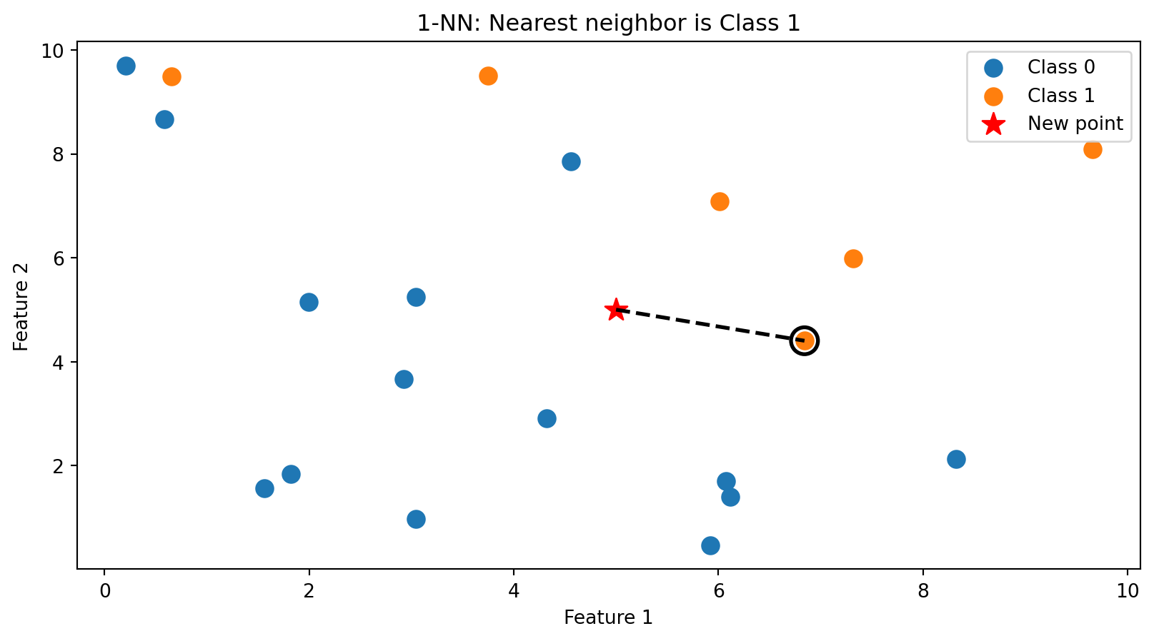
k-NN in Action: k = 1
With \(k = 1\), we classify based on the single closest training point. The new point (star) is assigned the class of its nearest neighbor (circled).
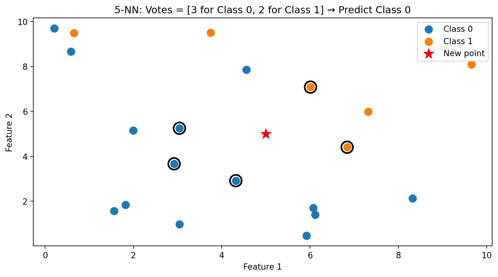
k-NN in Action: k = 5
With \(k = 5\), we take a majority vote among the 5 nearest neighbors (circled). This is more robust than using just one neighbor.
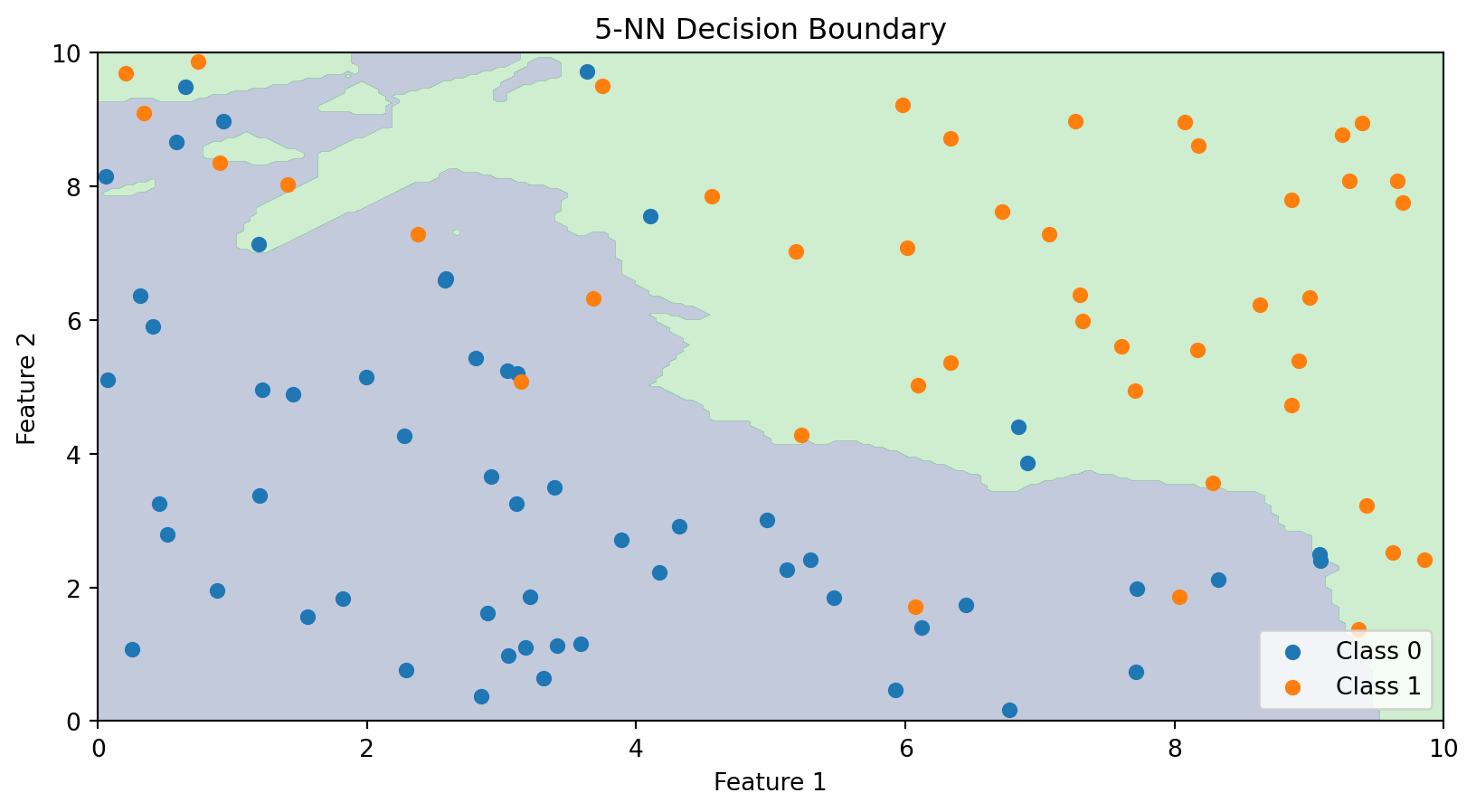
The Decision Boundary of k-NN
Unlike linear classifiers, k-NN doesn’t explicitly compute a decision boundary. But we can visualize what the boundary looks like by classifying every point in the feature space.
The k-NN decision boundary is nonlinear and adapts to the local density of data. It naturally forms complex shapes without us specifying any functional form.
The Role of k: Bias-Variance Tradeoff
The choice of \(k\) is crucial:
Small k (e.g., k = 1):
Boundary closely follows the training data
Very flexible—can capture complex patterns
High variance, low bias
Risk of overfitting (sensitive to noise)
Large k (e.g., k = 100):
Boundary is smoother
Less flexible—averages over many neighbors
Low variance, high bias
Risk of underfitting (misses local patterns)
This is the bias-variance tradeoff we’ve seen before. We need to choose \(k\) that balances these concerns.
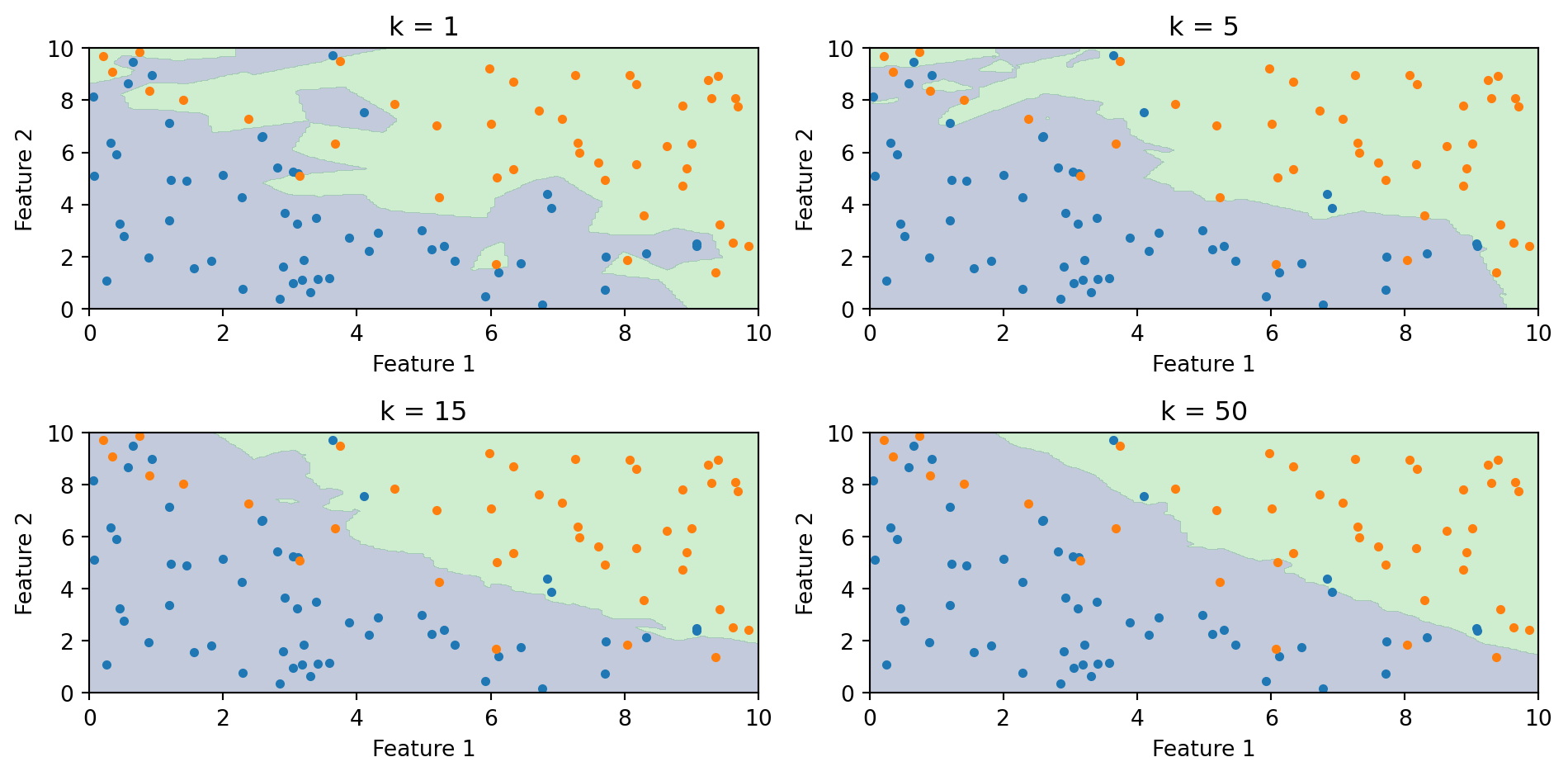
Effect of k on the Decision Boundary
As \(k\) increases, the boundary becomes smoother. With \(k = 1\), every training point gets its own region. With large \(k\), the boundary approaches the overall majority class.
Choosing k with Cross-Validation
How do we choose \(k\)? Use cross-validation (from Lecture 5):
Split training data into folds
For each candidate value of \(k\):
Fit k-NN on training folds
Evaluate accuracy on validation fold
Choose \(k\) that maximizes cross-validated accuracy
A common rule of thumb: \(k < \sqrt{n}\) where \(n\) is the sample size. But cross-validation is more reliable.
from sklearn.neighbors import KNeighborsClassifierfrom sklearn.model_selection import cross_val_scoreimport numpy as np# Try different values of kk_values =range(1, 31)cv_scores = []for k in k_values: knn = KNeighborsClassifier(n_neighbors=k) scores = cross_val_score(knn, X_train, y_train, cv=5) cv_scores.append(scores.mean())best_k = k_values[np.argmax(cv_scores)]print(f"Best k: {best_k} with CV accuracy: {max(cv_scores):.3f}")
Best k: 19 with CV accuracy: 0.850
k-NN: Advantages and Disadvantages
Advantages:
Simple to understand and implement
No training phase (just store the data)
Naturally handles multi-class problems
Can capture complex, nonlinear boundaries
No assumptions about the data distribution
Disadvantages:
Slow at prediction time—must compute distances to all training points
Doesn’t work well in high dimensions (“curse of dimensionality”)
Sensitive to irrelevant features (all features contribute to distance)
Requires feature scaling
For large datasets, approximate nearest neighbor methods can speed up k-NN, but it remains computationally intensive.
The Curse of Dimensionality
k-NN relies on distance, and distance breaks down in high dimensions. Three related problems:
The space becomes sparse. In 1D, 100 points cover the range well. In 2D, the same 100 points are scattered across a plane. In 50D, they’re lost in a vast empty space. The amount of data you need to “fill” the space grows exponentially with \(p\).
You need more data to have local neighbours. If the space is mostly empty, the \(k\) “nearest” neighbours may be far away — and far-away neighbours aren’t informative about the local structure.
Distances become less informative. Euclidean distance sums \(p\) squared differences. As \(p\) grows, all these sums converge to roughly the same value (law of large numbers). The nearest and farthest neighbours end up almost the same distance away, so “nearest” stops meaning much.
Part V: Decision Trees
The Intuition Behind Decision Trees
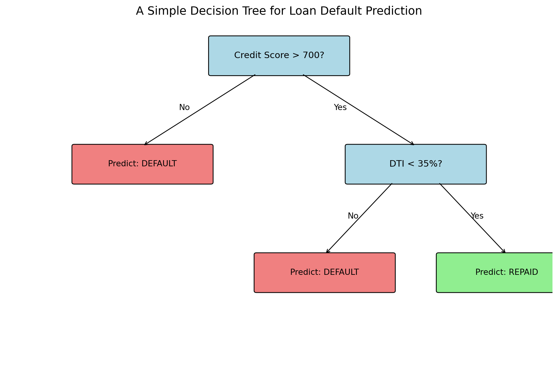
Decision trees mimic how humans make decisions: a series of yes/no questions.
Consider a loan officer evaluating an application:
Is the credit score above 700?
If no → High risk, deny
If yes → Continue…
Is the debt-to-income ratio below 35%?
If no → Medium risk, deny
If yes → Low risk, approve
Each question splits the population into subgroups, and we make predictions based on which group an observation falls into.
Decision trees automate this process: they learn which questions to ask and in what order.
Anatomy of a Decision Tree
Terminology:
Root node: The first split (top of the tree)
Internal nodes: Decision points that split the data
Leaf nodes: Terminal nodes that make predictions
Depth: The number of splits from root to leaf
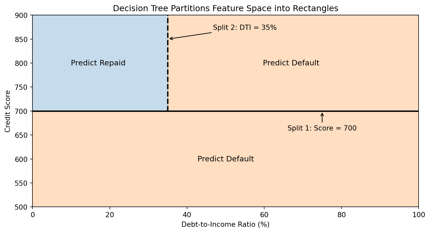
How Trees Partition the Feature Space
Each split in a decision tree divides the feature space with an axis-aligned boundary (parallel to one axis).
The tree creates rectangular regions. Each leaf corresponds to one region, and all observations in that region get the same prediction.
The Decision Tree Algorithm: Recursive Partitioning
The Goal: Build a tree that makes good predictions.
The Approach: Greedy, recursive partitioning.
Start with all training data at the root
Find the best split—the feature and threshold that best separates the classes
Split the data into two groups based on this rule
Recursively apply steps 2-3 to each group
Stop when a stopping criterion is met (e.g., minimum samples per leaf, maximum depth)
The key question: How do we define “best” split?
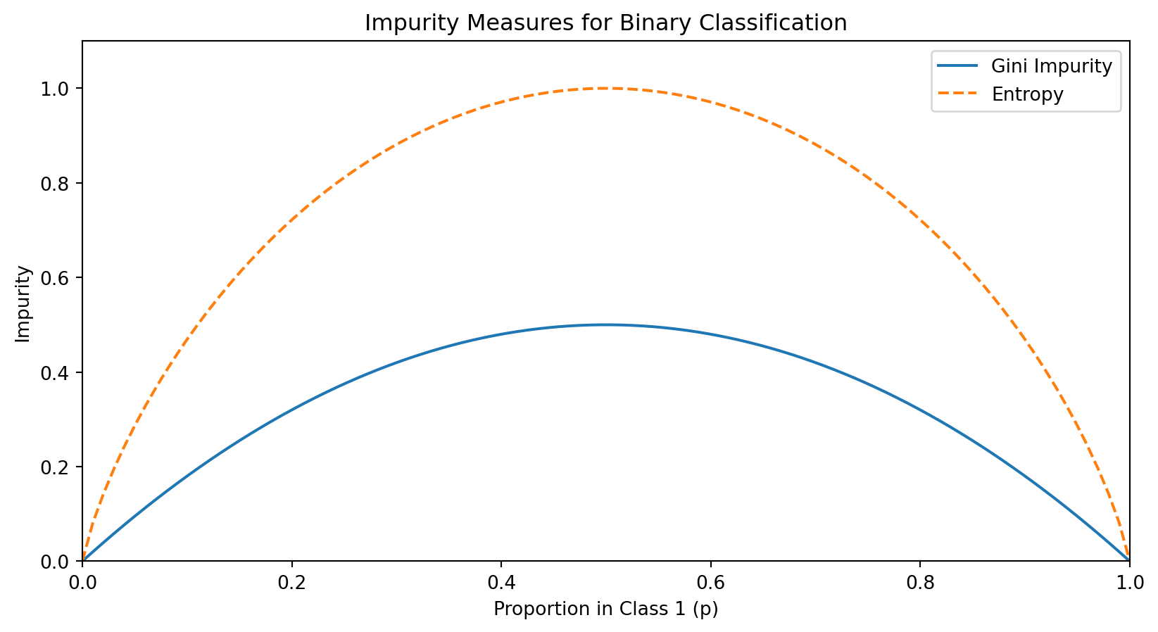
Measuring Split Quality: Impurity
A good split should create child nodes that are more “pure” than the parent—ideally, each child contains only one class.
We measure impurity—how mixed the classes are in a node. A pure node (all one class) has impurity = 0.
For a node with \(n\) observations where \(p_c\) is the proportion belonging to class \(c\):
We’d compute this for all possible features and thresholds, then choose the split with highest gain.
For Continuous Features: Finding the Best Threshold
For a continuous feature (like credit score), we need to find the best threshold for splitting.
Algorithm:
Sort the observations by the feature value
Consider each unique value as a potential threshold
For each threshold, compute the information gain
Choose the threshold with the highest gain
If there are \(n\) unique values, we evaluate up to \(n-1\) possible splits for that feature. This is computationally tractable because we can update class counts incrementally as we move through sorted values.
Building a Tree in Python
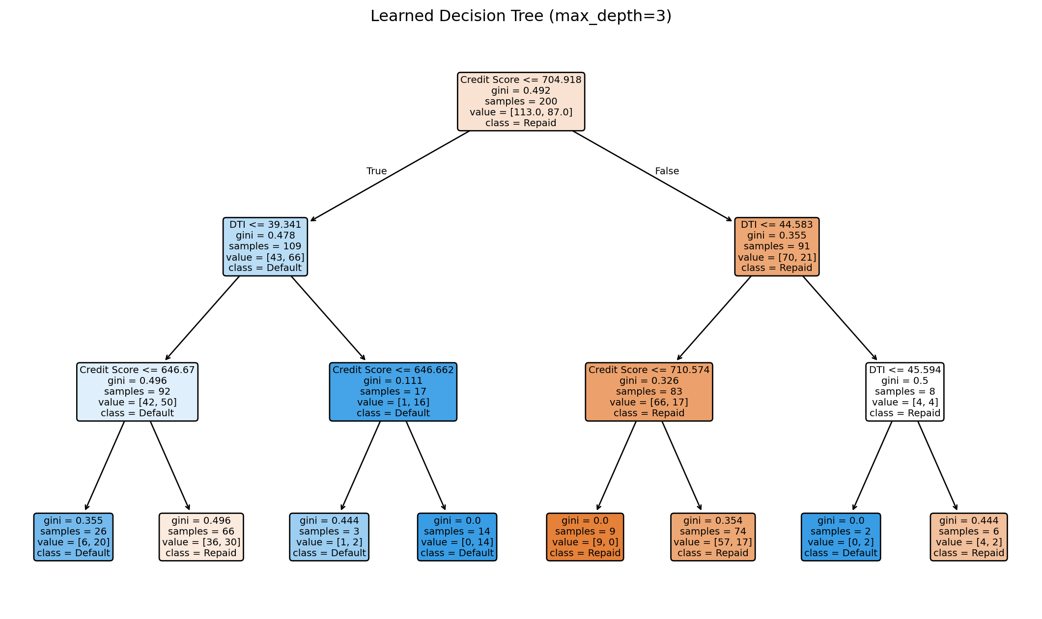
from sklearn.tree import DecisionTreeClassifierimport numpy as np# Generate sample datanp.random.seed(42)n =200credit_score = np.random.normal(700, 50, n)dti = np.random.normal(30, 10, n)X_tree = np.column_stack([credit_score, dti])# Default probability depends on both featuresprob_default =1/ (1+ np.exp(0.02* (credit_score -680) -0.05* (dti -35)))y_tree = (np.random.random(n) < prob_default).astype(int)# Fit decision treetree = DecisionTreeClassifier(max_depth=3, random_state=42)tree.fit(X_tree, y_tree)print(f"Tree depth: {tree.get_depth()}")print(f"Number of leaves: {tree.get_n_leaves()}")print(f"Training accuracy: {tree.score(X_tree, y_tree):.3f}")
Tree depth: 3
Number of leaves: 8
Training accuracy: 0.720
Visualizing the Learned Tree
The tree learns splits automatically from the data. Each node shows the split condition, impurity, sample count, and class distribution.
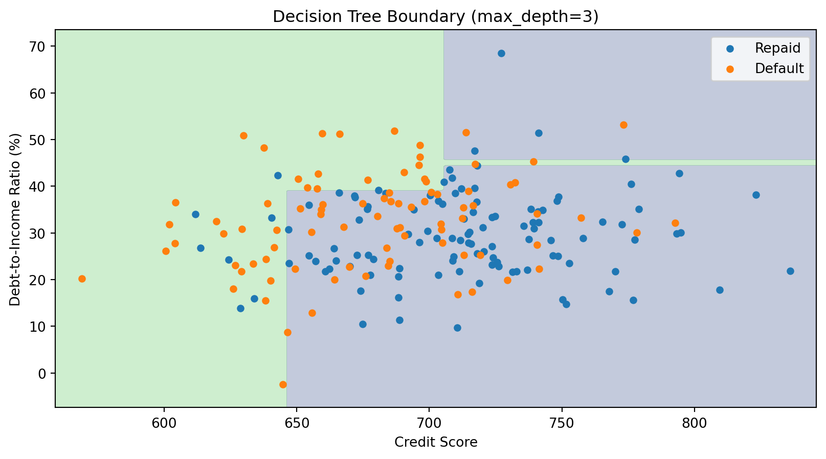
The Decision Boundary of a Tree
Decision tree boundaries are always axis-aligned rectangles—combinations of horizontal and vertical lines. This is a limitation compared to k-NN’s curved boundaries.
Controlling Tree Complexity
Deep trees can overfit—they memorize the training data perfectly but fail on new data.
Strategies to prevent overfitting:
Pre-pruning: Stop growing before the tree becomes too complex
max_depth: Maximum tree depth
min_samples_split: Minimum samples required to split a node
min_samples_leaf: Minimum samples required in a leaf
Post-pruning: Grow a full tree, then remove branches that don’t help
ccp_alpha: Cost-complexity pruning parameter
These hyperparameters are chosen via cross-validation.
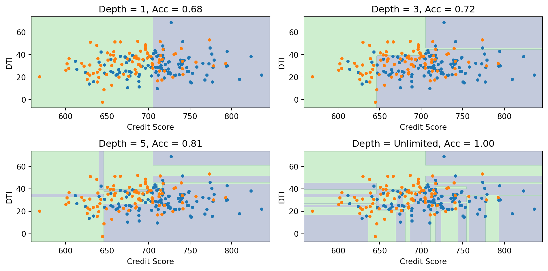
Effect of Tree Depth
Deeper trees create more complex boundaries. With unlimited depth, the tree can achieve 100% training accuracy but likely overfits.
Decision Trees: Advantages and Disadvantages
Advantages:
Easy to interpret and explain (white-box model)
Handles both numeric and categorical features
Requires little data preprocessing (no scaling needed)
Can capture interactions between features
Fast prediction
Disadvantages:
Axis-aligned boundaries only (can’t capture diagonal boundaries efficiently)
High variance—small changes in data can produce very different trees
Prone to overfitting without regularization
Greedy algorithm may not find globally optimal tree
The high variance problem is addressed by ensemble methods (Random Forests, Gradient Boosting)—we’ll revisit decision trees as building blocks for these in the next lecture.
Part VI: Evaluating Classification Models
Beyond Accuracy
For regression, we use MSE or \(R^2\) to measure performance.
For classification, accuracy (% correct) is the obvious metric:
Precision: Of those we predicted positive, how many actually are? \[\text{Precision} = \frac{TP}{TP + FP}\]
Recall (Sensitivity): Of the actual positives, how many did we catch? \[\text{Recall} = \frac{TP}{TP + FN}\]
Specificity: Of the actual negatives, how many did we correctly identify? \[\text{Specificity} = \frac{TN}{TN + FP}\]
False Positive Rate: Of actual negatives, how many did we wrongly call positive? \[\text{FPR} = \frac{FP}{TN + FP} = 1 - \text{Specificity}\]
Credit Default: Confusion Matrix
from sklearn.metrics import confusion_matrix, classification_report# Using our credit default data with logistic regressiony_pred = log_reg.predict(X)# Confusion matrixcm = confusion_matrix(default, y_pred)print("Confusion Matrix:")print(f" Predicted No Predicted Yes")print(f" Actual No {cm[0,0]:5d}{cm[0,1]:5d}")print(f" Actual Yes {cm[1,0]:5d}{cm[1,1]:5d}")
Confusion Matrix:
                  Predicted No  Predicted Yes
  Actual No          961793          5207
  Actual Yes         19202         13798
Lowering the threshold from 0.5 to 0.1 dramatically increases recall (catching defaults) at the cost of more false positives.
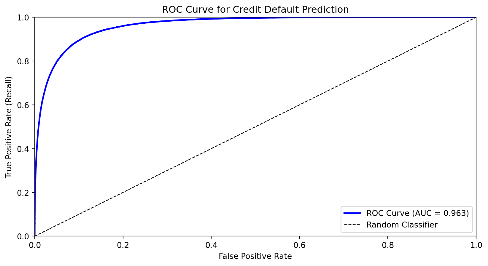
The ROC Curve
The Receiver Operating Characteristic (ROC) curve shows the trade-off between true positive rate (recall) and false positive rate across all thresholds.
X-axis: False Positive Rate (FPR)
Y-axis: True Positive Rate (TPR = Recall)
As we lower the threshold:
We move from bottom-left (predict nothing positive) toward top-right (predict everything positive)
Good classifiers hug the top-left corner
Area Under the ROC Curve (AUC)
The Area Under the Curve (AUC) summarizes the ROC curve in a single number:
AUC = 1.0: Perfect classifier
AUC = 0.5: Random guessing (diagonal line)
AUC < 0.5: Worse than random (predictions inverted)
Interpretation: AUC is the probability that a randomly chosen positive example is ranked higher than a randomly chosen negative example.
from sklearn.metrics import roc_auc_scoreauc = roc_auc_score(default, prob_pred)print(f"AUC for credit default model: {auc:.3f}")
AUC for credit default model: 0.963
AUC is useful for comparing models because it’s threshold-independent—it measures the model’s ability to rank observations correctly.
Choosing the Optimal Threshold
The “best” threshold depends on the costs of different errors:
Cost of false negative (missing a default): \(c_{FN}\)
Cost of false positive (false alarm): \(c_{FP}\)
If missing defaults is very costly (e.g., the bank loses the loan amount), we want a lower threshold to maximize recall.
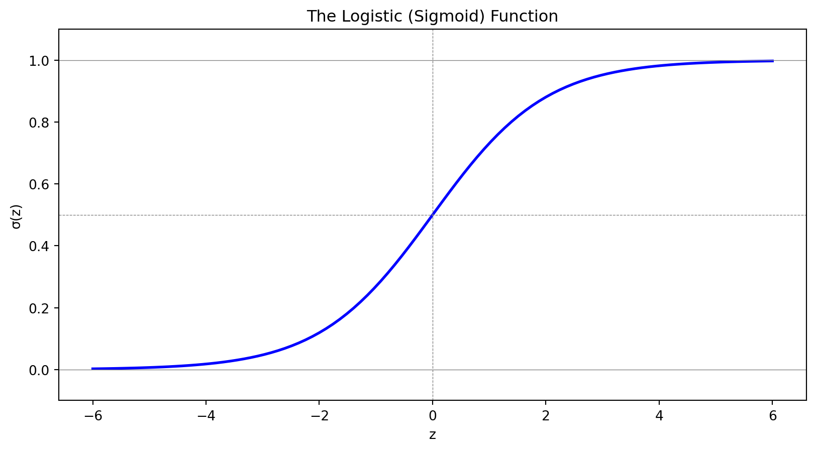
Logistic regression uses the sigmoid function to model probabilities:
Outputs are always in (0, 1)
Coefficients measure effect on log-odds
Decision boundary is linear; can be extended with feature engineering
Can be regularized (Lasso) for variable selection
k-Nearest Neighbors classifies based on majority vote among nearby training points:
Flexible, curved decision boundaries without specifying functional form
Requires feature scaling; struggles in high dimensions
No training phase, but slow at prediction time
Decision trees recursively partition feature space with axis-aligned splits:
Highly interpretable; handles mixed feature types
Prone to overfitting and high variance
Building blocks for ensemble methods (next lecture)
Evaluation Metrics
Accuracy can be misleading with imbalanced classes.
The confusion matrix breaks down predictions into TP, FP, TN, FN.
Precision (of predicted positives, how many are correct?) and Recall (of actual positives, how many did we catch?) capture different aspects of performance.
The ROC curve shows the trade-off across all thresholds.
AUC summarizes discriminative ability in a single number.
The optimal threshold depends on the costs of different types of errors.
Next Lecture
Lecture 8: Ensemble Methods
Decision trees have high variance—small changes in data can produce very different trees. next lecture we’ll see how to fix this.
Random Forests: Average many trees, each trained on random subsets
Gradient Boosting: Build trees sequentially, each correcting previous errors
XGBoost: Industrial-strength boosting used in finance and competitions
Ensemble methods combine many weak learners into a strong learner, dramatically reducing variance while maintaining flexibility.
References
Cover, T., & Hart, P. (1967). Nearest neighbor pattern classification. IEEE Transactions on Information Theory, 13(1), 21-27.
Breiman, L., Friedman, J., Stone, C. J., & Olshen, R. A. (1984). Classification and Regression Trees. CRC Press.
Hastie, T., Tibshirani, R., & Friedman, J. (2009). The Elements of Statistical Learning (2nd ed.). Springer. Chapters 4, 9, 13.
James, G., Witten, D., Hastie, T., & Tibshirani, R. (2021). An Introduction to Statistical Learning (2nd ed.). Springer. Chapter 4.
Quinlan, J. R. (1986). Induction of decision trees. Machine Learning, 1(1), 81-106.
Appendix: Linear Discriminant Analysis
Why Another Classifier?
Clustering (Lecture 5)
Logistic Regression
LDA
Type
Unsupervised
Supervised
Supervised
Labels
Unknown — discover them
Known — learn a boundary
Known — learn distributions
Strategy
Assume each group is a distribution; find the groups
Directly model \(P(y \mid \mathbf{x})\)
Model \(P(\mathbf{x} \mid y)\) per class, then apply Bayes’ theorem
LDA is the supervised version of the distributional thinking you used in clustering: instead of discovering groups, you already know them and want to learn what makes each group different.
In practice, LDA and logistic regression often give similar answers — the value is in understanding both ways of thinking about classification.
A Different Approach: Bayes’ Theorem
Logistic regression directly models \(P(y | \mathbf{x})\)—the probability of the class given the features.
Discriminant analysis takes a different approach using Bayes’ theorem:
\[P(y = k | \mathbf{x}) = \frac{P(\mathbf{x} | y = k) \cdot P(y = k)}{P(\mathbf{x})}\]
\(\boldsymbol{\mu}_k\) is the mean of class \(k\) (different for each class)
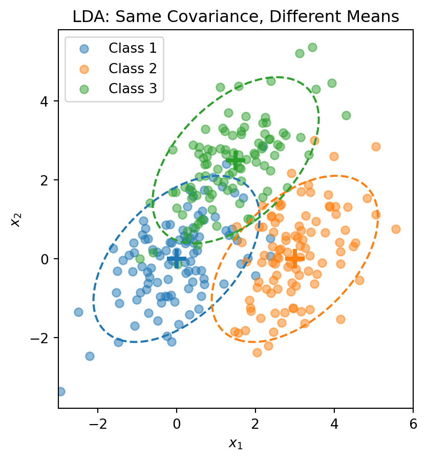
\(\boldsymbol{\Sigma}\) is the covariance matrix (same for all classes — this is the key assumption!)
Each class is a normal “blob” centered at \(\boldsymbol{\mu}_k\), but all classes share the same shape (covariance).
Visualizing the LDA Assumption
The dashed ellipses show the 95% probability contours—they have the same shape (orientation and spread) but different centers.
The LDA Discriminant Function
Start with the posterior from Bayes’ theorem:
\[P(y = k \,|\, \mathbf{x}) = \frac{f_k(\mathbf{x}) \pi_k}{\sum_{j=1}^{K} f_j(\mathbf{x}) \pi_j}\]
Taking the log and plugging in the normal density:
\[\ln P(y = k \,|\, \mathbf{x}) = \ln f_k(\mathbf{x}) + \ln \pi_k - \underbrace{\ln \sum_{j} f_j(\mathbf{x}) \pi_j}_{\text{same for all } k}\]
The normal density gives \(\ln f_k(\mathbf{x}) = -\frac{p}{2}\ln(2\pi) - \frac{1}{2}\ln|\boldsymbol{\Sigma}| - \frac{1}{2}(\mathbf{x} - \boldsymbol{\mu}_k)'\boldsymbol{\Sigma}^{-1}(\mathbf{x} - \boldsymbol{\mu}_k)\).
The first two terms don’t depend on \(k\) (shared covariance!). Expanding the quadratic and dropping terms that don’t depend on \(k\), we get the discriminant function:
This is a scalar—one number for each class \(k\). We classify \(\mathbf{x}\) to the class with the largest discriminant: \(\hat{y} = \arg\max_k \delta_k(\mathbf{x})\).
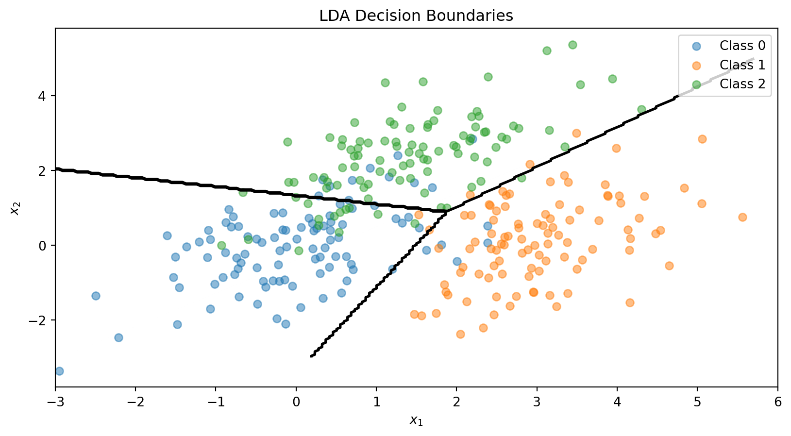
The discriminant function is linear in \(\mathbf{x}\)—that’s why it’s called Linear Discriminant Analysis.
The LDA Decision Boundary
The decision boundary between classes \(k\) and \(\ell\) is where:
The pooled covariance averages within-class covariances, weighted by class size.
The LDA Recipe
LDA
Model
Each class \(k\) is a multivariate normal: \(\mathbf{x} \mid y = k \;\sim\; \mathcal{N}(\boldsymbol{\mu}_k,\, \boldsymbol{\Sigma})\)
Parameters
Priors \(\hat{\pi}_k = n_k / n\), means \(\hat{\boldsymbol{\mu}}_k\), pooled covariance \(\hat{\boldsymbol{\Sigma}}\)
“Loss function”
Not a loss function — parameters are estimated directly from the data (sample proportions, sample means, pooled covariance)
Classification rule
Assign \(\mathbf{x}\) to the class with the largest discriminant \(\delta_k(\mathbf{x})\)
No optimization loop, no gradient descent. LDA computes its parameters in closed form — plug in the training data and you’re done.
This is fundamentally different from logistic regression, which iteratively searches for the coefficients that minimize cross-entropy loss.
LDA in Python
from sklearn.discriminant_analysis import LinearDiscriminantAnalysis# Combine the 3-class dataX_lda = np.vstack([X1, X2, X3])y_lda = np.array([0] * n_per_class + [1] * n_per_class + [2] * n_per_class)# Fit LDAlda = LinearDiscriminantAnalysis()lda.fit(X_lda, y_lda)print("LDA Class Means:")for k inrange(3):print(f" Class {k}: {lda.means_[k]}")print(f"\nClass Priors: {lda.priors_}")
LDA Class Means:
  Class 0: [ 0.00962094 -0.02608294]
  Class 1: [3.00835928 0.12294623]
  Class 2: [1.40152169 2.3715806 ]

Class Priors: [0.33333333 0.33333333 0.33333333]