Every model we have built so far takes numbers as input — returns, prices, financial ratios. But the vast majority of information produced in financial markets is text: earnings calls, analyst reports, news articles, SEC filings, social media posts.
Today we learn how to turn text into numbers so that our ML toolkit can work with it.
Today’s roadmap:
Text as data: Why text matters for finance, and the challenge of representing it numerically
Bag of words: The simplest text representation — word counts
TF-IDF: From raw counts to importance-weighted representations
Sentiment analysis: Dictionary-based and data-driven approaches for measuring tone
Topic modeling: Discovering latent themes with Latent Dirichlet Allocation (LDA)
Similarity and embeddings: Cosine similarity, Word2Vec, and contextual embeddings
Large language models: How modern NLP builds on everything above
Part I: Text as Data
Why Text in Finance?
Financial text is generated constantly: earnings call transcripts, 10-K filings, analyst reports, central bank minutes, financial news, Twitter/Reddit posts. Humans have always read these to form views about companies and markets. The question is whether machines can do it systematically.
Three reasons text data matters:
Scale: A single quarter produces thousands of earnings call transcripts. No human can read them all in real time.
Structure: Text often contains forward-looking information — management guidance, risk disclosures, tone shifts — that is not captured in historical price data.
Speed: Algorithmic systems can process a news article in milliseconds, well before most human traders react.
The finance literature has shown that text-derived signals predict returns, volatility, and corporate events (Tetlock 2007, Loughran and McDonald 2011, Ke, Kelly, and Xiu 2019).
The Challenge: Text is Ultra-High Dimensional
To apply any ML model, we need a numerical representation of text — a vector \(\mathbf{x} \in \mathbb{R}^p\) for each document.
The problem is that \(p\) is enormous. The Oxford English Dictionary lists roughly 170,000 English words in current use (OED 2nd Edition, 1989). After cleaning, the vocabulary for a financial corpus can be very large. Each document becomes a point in a space with tens of thousands of dimensions, and most coordinates are zero.
This is exactly the kind of high-dimensional, sparse data that ML is designed for. The tools we have studied — regularization (Lecture 5), clustering (Lecture 4), classification (Lectures 7–8) — all become relevant here.
The pipeline for any text-based analysis:
Collect raw text (the corpus)
Clean and preprocess (lowercase, remove punctuation, stem/lemmatize, remove stop words)
Represent numerically (bag of words, TF-IDF, embeddings)
Model (classification, regression, clustering, topic modeling)
A Running Example
Throughout this lecture we will work with a small corpus of Wall Street Journal articles from 2026, covering different financial topics: gas prices, European monetary policy, a food industry merger, prediction market regulation, and a bank settlement.
Here is the opening of one article:
Gas Just Hit $4 a Gallon. Is That Really as Bad as It Sounds? — Wall Street Journal, March 31, 2026
There is an argument that Americans shouldn’t worry much about $4 gasoline. The people filling their tanks might not be convinced by it. The average price for a gallon of regular gasoline hit $4.02 on Tuesday, according to AAA. That was the first time it has been above $4 since August 2022, when the world was still struggling to absorb the oil shock from the Russia-Ukraine war.
Each article uses only a small fraction of the English vocabulary. This extreme sparsity — most words do not appear in any given document — is typical of text data.
Loading the Corpus
import os# Read all articles from our corpuscorpus = {}for filename insorted(os.listdir("10_text")):if filename.endswith(".txt"):withopen(f"10_text/{filename}") as f: corpus[filename] = f.read()# Display article names and word countsfor name, text in corpus.items(): words = text.split()print(f"{name:45s}{len(words):>4} words")
bofasettlement_wsj.txt                         538 words
europemonetarypolicy_wsj.txt                   878 words
foodmerger_wsj.txt                             798 words
gas_wsj.txt                                    643 words
sportsbettingprediction_wsj.txt                646 words
Part II: Bag of Words
The Bag of Words Representation
The simplest way to represent a document numerically: count how many times each word appears.
Suppose our dictionary has \(V\) words. For each document \(d\), we create a vector \(\mathbf{x}_d \in \mathbb{R}^V\) where entry \(j\) is the count of word \(j\) in document \(d\).
Consider the headline: “Gas prices rise as energy prices rise”
If our dictionary is {gas:1, prices:2, rise:3, as:4, energy:5}, then the bag-of-words (BOW) vector is:
\[\mathbf{x} = (1, 2, 2, 1, 1)\]
“Prices” has count 2 because it appears twice, and so does “rise.” The representation completely ignores the order of words — “prices rise” and “rise prices” produce the same vector. That is why it is called a “bag” of words: imagine dumping all the words into a bag and shaking them up.
N-Grams: Capturing Word Order
One way to partially recover word order: instead of counting individual words, count sequences of consecutive words.
Unigram (1-gram): individual words — “gas”, “prices”, “rise”
Bigrams distinguish “prices rise” from “rise prices.” The phrase “prices rise” describes inflation, while “rise prices” means something different (to increase prices). Word order matters for meaning, and bigrams partially capture it.
Formally, an n-gram model decomposes the probability of a word sequence as:
The trade-off: n-grams are more expressive but the dictionary size explodes. With \(V\) unique words, there are up to \(V^2\) bigrams and \(V^3\) trigrams. In practice, most text analyses use unigrams or unigrams + bigrams.
Text Preprocessing
Before building the term-document matrix, we clean the raw text. Each step reduces the vocabulary size and removes noise.
Step 1: Lowercase
“IBM” and “ibm” and “Ibm” should all be the same token. Convert everything to lowercase. (Exception: sometimes you keep proper nouns like ticker symbols.)
Step 2: Remove punctuation and numbers
Commas, periods, dollar signs, and standalone numbers (“13.5%”) typically add noise rather than signal.
Step 3: Remove stop words
Stop words are high-frequency words with little semantic content: “the”, “a”, “is”, “and”, “of”, “to”, “in”, etc. The NLTK English stop word list contains 179 words. Removing them can cut 30–50% of all tokens.
Step 4: Stemming or lemmatization
Reduce words to their root form so that variants count together:
After preprocessing, we arrange the word counts into a term-document matrix\(\mathbf{X} \in \mathbb{R}^{D \times V}\), where \(D\) is the number of documents and \(V\) is the vocabulary size.
Each row is one document. Each column is one word. Entry \(x_{dj}\) is the count of word \(j\) in document \(d\).
This matrix is almost always very sparse: most entries are zero because any given document uses only a tiny fraction of the full vocabulary. For a corpus of 10,000 news articles with a 50,000-word vocabulary, the matrix has 500 million entries, but 99%+ of them are zero.
In Python, sklearn.feature_extraction.text.CountVectorizer builds this matrix directly from raw text, handling tokenization, stop word removal, and n-gram construction in one step.
Building the Term-Document Matrix in Python
from sklearn.feature_extraction.text import CountVectorizerimport pandas as pd# Build the term-document matrix (removing English stop words)vectorizer = CountVectorizer(stop_words="english")X = vectorizer.fit_transform(corpus.values())# Short names for displaynames = [n.replace("_wsj.txt", "").replace(".txt", "") for n in corpus.keys()]print(f"Documents: {X.shape[0]}")print(f"Vocabulary size: {X.shape[1]}")print(f"Non-zero entries: {X.nnz} out of {X.shape[0] * X.shape[1]}")print(f"Sparsity: {1- X.nnz / (X.shape[0] * X.shape[1]):.1%}")
Documents:        5
Vocabulary size:  1090
Non-zero entries: 1275 out of 5450
Sparsity:         76.6%
Examining Word Counts
# Convert to a DataFramewords = vectorizer.get_feature_names_out()df_bow = pd.DataFrame(X.toarray(), index=names, columns=words)# Pick some words that should differ across articlessample_words = ["prices", "oil", "gas", "rate", "inflation","bank", "merger", "betting", "lawsuit"]sample_words = [w for w in sample_words if w in df_bow.columns]df_bow[sample_words]
prices
oil
gas
rate
inflation
bank
merger
betting
lawsuit
bofasettlement
0
0
0
0
0
14
0
0
11
europemonetarypolicy
14
4
3
12
9
6
0
0
0
foodmerger
3
0
0
0
0
0
2
0
0
gas
9
1
1
0
6
0
0
0
0
sportsbettingprediction
0
0
0
0
0
0
0
4
1
Each row is an article, each column is a word. Most entries are zero — a word like “oil” appears frequently in the gas article but not at all in the bank settlement article.
Part III: From Counts to Weights — TF-IDF
The Problem with Raw Counts
Raw word counts treat all words equally. But some words are more informative than others.
Consider two words that both appear 5 times in an earnings call transcript:
“revenue” — appears in nearly every earnings call. High count, but not distinctive.
“restructuring” — appears in only a few transcripts. High count and distinctive.
The word “restructuring” tells us much more about what makes this particular document different from others. We want a weighting scheme that rewards words that are frequent in this document but rare across the corpus.
TF-IDF: Term Frequency–Inverse Document Frequency
TF-IDF is the standard weighting scheme that addresses this problem. It has two components:
Term Frequency (TF): How often does word \(j\) appear in document \(d\)?
\[\text{TF}(j, d) = \frac{\text{count of word } j \text{ in document } d}{\text{total words in document } d}\]
This normalizes for document length — a 1,000-word article with 5 occurrences of “revenue” and a 100-word article with 5 occurrences of “revenue” are not the same.
Inverse Document Frequency (IDF): How rare is word \(j\) across all documents?
\[\text{IDF}(j) = \ln\left(\frac{D}{D_j}\right)\]
where \(D\) is the total number of documents and \(D_j\) is the number of documents containing word \(j\). Words appearing in every document get IDF \(= \ln(1) = 0\). Words appearing in only one document get the maximum IDF \(= \ln(D)\).
The TF-IDF score is high when a word is frequent in the current document and rare across the corpus. It is low when the word is common everywhere or when it barely appears in the current document.
We can see this directly in our corpus. The code below computes TF, IDF, and TF-IDF by hand for three words in the gas article:
import numpy as np# Pick three words to compare in the gas articletarget_words = ["prices", "gasoline", "gallon"]# Get the gas article's row indexdoc_idx = names.index("gas")n_docs = X.shape[0]for word in target_words:if word notin words:continue col =list(words).index(word) count = X[doc_idx, col] # raw count in this article total_words = X[doc_idx].sum() # total words in this article docs_with_word = (X[:, col].toarray() >0).sum() # docs containing this word tf = count / total_words idf = np.log(n_docs / docs_with_word) tfidf = tf * idfprint(f'"{word:10s}" count={count} docs_with_word={docs_with_word}/{n_docs}'f' TF={tf:.4f} IDF={idf:.2f} TF-IDF={tfidf:.4f}')
Words that appear in many articles get a low IDF (they are not distinctive). Words concentrated in one article get a high IDF and therefore a high TF-IDF score.
In Python, sklearn.feature_extraction.text.TfidfVectorizer builds the full TF-IDF matrix directly and is typically the default starting point for any text analysis.
TF-IDF in Python
from sklearn.feature_extraction.text import TfidfVectorizer# Build the TF-IDF matrixtfidf = TfidfVectorizer(stop_words="english")X_tfidf = tfidf.fit_transform(corpus.values())# Compare TF-IDF scores for the same words as beforewords_tfidf = tfidf.get_feature_names_out()df_tfidf = pd.DataFrame(X_tfidf.toarray(), index=names, columns=words_tfidf)df_tfidf[sample_words].round(3)
prices
oil
gas
rate
inflation
bank
merger
betting
lawsuit
bofasettlement
0.000
0.000
0.000
0.000
0.000
0.343
0.000
0.000
0.270
europemonetarypolicy
0.263
0.091
0.068
0.337
0.204
0.136
0.000
0.000
0.000
foodmerger
0.059
0.000
0.000
0.000
0.000
0.000
0.059
0.000
0.000
gas
0.192
0.026
0.026
0.000
0.154
0.000
0.000
0.000
0.000
sportsbettingprediction
0.000
0.000
0.000
0.000
0.000
0.000
0.000
0.121
0.025
Compare this to the raw counts above. Words that are common across many articles (like “prices”) get lower TF-IDF scores, while words unique to one article (like “betting” or “lawsuit”) get higher scores.
Part IV: Sentiment Analysis
What is Sentiment Analysis?
Sentiment analysis tries to measure the tone of a document — is it positive, negative, or neutral?
In finance, this is directly useful:
Does an earnings call transcript sound optimistic or pessimistic?
Is a news article about a company positive or negative?
Is the tone of Fed minutes hawkish or dovish?
The simplest approach uses pre-built sentiment dictionaries: lists of words pre-classified as positive or negative. Count the positive and negative words, and compute a score.
Dictionary-Based Sentiment: Loughran and McDonald (2011)
A widely used finance-specific sentiment dictionary was developed by Loughran and McDonald (2011). They pointed out that general-purpose sentiment dictionaries (like the Harvard General Inquirer) misclassify many financial terms.
For example, the word “liability” is negative in everyday English but routine in financial text. The word “outstanding” is positive in everyday English but means “currently owed” in financial text (“outstanding shares”, “outstanding debt”).
The Loughran-McDonald dictionary contains six word lists tailored to 10-K filings:
where \(N_d^+\) is the count of positive words and \(N_d^-\) is the count of negative words. This score ranges from \(-1\) (entirely negative) to \(+1\) (entirely positive).
An alternative normalization divides by the total word count in the document:
\[\text{Sentiment}_d = \frac{N_d^+ - N_d^-}{\text{Total words in } d}\]
This adjusts for document length and allows comparison across short news articles and long 10-K filings.
Sentiment Scoring in Python
We can apply a simple dictionary approach to our corpus. The word lists below are a small sample inspired by Loughran and McDonald (2011):
# Small finance-oriented sentiment word listsnegative = {"loss", "decline", "fell", "fall", "risk", "lawsuit", "penalty","recession", "inflation", "debt", "default", "failure", "hurt","erode", "drop", "sank", "slipped", "charges", "convicted","tumbled", "worried", "weary", "disrupted", "ban", "illegal"}positive = {"growth", "gain", "profit", "improve", "success", "benefit","rose", "growing", "boost", "excelled", "opportunity", "strong"}# Score each articlefor name, text in corpus.items(): tokens = text.lower().split() neg =sum(1for w in tokens if w in negative) pos =sum(1for w in tokens if w in positive) total = pos + negif total >0: score = (pos - neg) / totalelse: score =0.0 label = name.replace("_wsj.txt", "").replace(".txt", "")print(f"{label:35s} pos={pos:2d} neg={neg:2d} score={score:+.2f}")
Dictionary-based sentiment is simple and interpretable, but has clear weaknesses:
Negation: “Revenue did not decline” contains the negative word “decline” but the sentence is actually positive. A simple word count misses this.
Context: “The risk of loss is minimal” — “risk” and “loss” are negative words, but the sentence is reassuring.
Sarcasm and nuance: “What a great quarter for shareholders” might be sarcastic in context.
Domain specificity: Even finance-specific dictionaries cannot cover every context. “Volatility” is negative for a risk manager but could be positive for an options trader.
Fixed vocabulary: Dictionaries do not adapt to new language. Financial jargon evolves — “meme stock” or “SPAC” would not appear in a dictionary built from 10-K filings.
These limitations motivate more sophisticated approaches: learning sentiment from data rather than specifying it in advance.
SESTM: Learning Sentiment from Data
Ke, Kelly, and Xiu (2019) developed SESTM — Sentiment Extraction via Screening and Topic Modeling — which learns which words carry sentiment from the data itself, rather than relying on a pre-built dictionary.
The approach has two stages:
Stage 1 — Screening: Of the many thousands of words in the vocabulary, most are irrelevant to sentiment. Screen for words whose frequency correlates with subsequent stock returns. This reduces the vocabulary from \(V\) to a much smaller set \(V_S\) of “sentiment-charged” words.
Stage 2 — Topic model: Model the screened word counts as a mixture of two topics: a positive topic \(O_+\) and a negative topic \(O_-\). Each document gets a sentiment score \(p_i \in [0, 1]\) based on how much it loads on the positive versus negative topic.
Recall that a Multinomial distribution models the outcome of drawing \(n\) items from a set of categories, each with a fixed probability — like rolling a weighted die \(n\) times and counting how often each face appears. Here, the “die” has one face per sentiment-charged word, and the probabilities come from a blend of the positive and negative topics:
\(d_{iS}\) is the vector of sentiment-charged word counts in article \(i\)
\(s_i\) is the total number of sentiment-charged words in article \(i\) (the number of “draws”)
\(O_+\) and \(O_-\) are probability vectors over the vocabulary — the positive and negative topics
\(p_i \in [0, 1]\) is the sentiment score: \(p_i\) close to 1 means the article’s words are drawn mostly from the positive topic, \(p_i\) close to 0 means mostly negative
The model estimates three things: the positive topic \(O_+\) (which words are associated with good news), the negative topic \(O_-\) (which words are associated with bad news), and a sentiment score \(p_i\) for every article. The topics \(O_+\) and \(O_-\) are estimated once from the entire corpus. The \(p_i\) are estimated separately for each article — they are the output of interest, giving each article a data-driven sentiment score without ever specifying a dictionary.
Applied to Dow Jones newswires (2004–2017), SESTM produces a daily long-short portfolio with a Sharpe ratio of 4.29 (equal-weighted) — substantially higher than dictionary-based approaches.
Part V: Topic Modeling
What is Topic Modeling?
Sentiment analysis reduces a document to a single number (positive/negative). But documents contain richer information. An earnings call might discuss revenue growth, cost cutting, regulatory risk, and new product launches — all in the same transcript.
Topic modeling is an unsupervised method that discovers the latent themes (topics) in a collection of documents. It answers: “What is this corpus about?” without any labels.
Recall from Lecture 4 that unsupervised learning discovers structure in data without labels. Topic modeling is the text equivalent of clustering: instead of grouping data points, we discover groups of words that tend to co-occur.
The most widely used topic model is Latent Dirichlet Allocation (LDA), introduced by Blei, Ng, and Jordan (2003). Despite the shared acronym, this LDA is unrelated to the Linear Discriminant Analysis from Lecture 7.
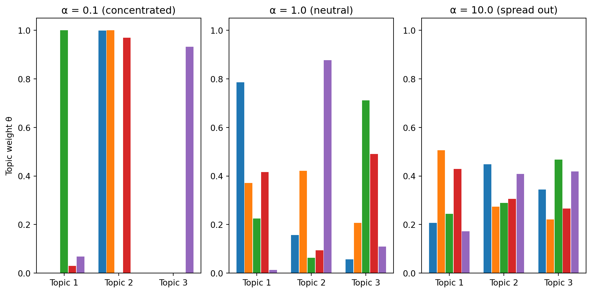
The Dirichlet Distribution
Before we can describe LDA, we need to understand the Dirichlet distribution — a distribution that generates probability vectors (vectors of non-negative numbers that sum to 1).
Suppose we have \(K = 3\) topics. A probability vector \(\boldsymbol{\theta} = (\theta_1, \theta_2, \theta_3)\) with \(\theta_1 + \theta_2 + \theta_3 = 1\) describes how much of each topic a document contains. The Dirichlet distribution is a way to randomly generate such vectors.
It has one parameter: \(\boldsymbol{\alpha} = (\alpha_1, \ldots, \alpha_K)\). When all \(\alpha_k\) are equal to some value \(\alpha\), this single number controls the concentration of the resulting vectors:
Small \(\alpha\) (e.g., 0.1): Most of the probability mass lands on one or two topics. Documents are “about” one thing.
\(\alpha = 1\): All probability vectors are equally likely — a uniform prior over mixtures.
Large \(\alpha\) (e.g., 10): The probability is spread roughly evenly across all topics. Documents are a balanced blend.
Visualizing the Dirichlet
import numpy as npimport matplotlib.pyplot as pltnp.random.seed(42)# Sample topic mixtures from Dirichlet with different alpha valuesfig, axes = plt.subplots(1, 3)topics = ["Topic 1", "Topic 2", "Topic 3"]for ax, alpha, title inzip(axes, [0.1, 1.0, 10.0], ["α = 0.1 (concentrated)", "α = 1.0 (neutral)", "α = 10.0 (spread out)"]):# Sample 5 documents' topic mixtures samples = np.random.dirichlet([alpha, alpha, alpha], size=5) x = np.arange(3)for i, theta inenumerate(samples): ax.bar(x + i *0.15, theta, width=0.14) ax.set_xticks(x +0.3) ax.set_xticklabels(topics) ax.set_ylim(0, 1.05) ax.set_title(title)axes[0].set_ylabel("Topic weight θ")plt.tight_layout()plt.show()
Each group of bars is one sampled document’s topic mixture. With small \(\alpha\), each document is dominated by a single topic. With large \(\alpha\), every document is a roughly equal blend. In practice, real text corpora tend to have small \(\alpha\) — most documents focus on a few topics, not all of them equally.
LDA: The Generative Story
LDA is a generative model — it tells a fictional story about how documents are created, then works backward to infer the hidden structure from the words we actually observe.
Suppose we have \(K\) topics and a vocabulary of \(V\) words. Each topic \(k\) has its own word distribution \(\boldsymbol{\phi}_k\) (phi) — a vector of \(V\) probabilities that sum to 1. For example, a “monetary policy” topic would put high probability on words like “rate”, “inflation”, “fed”, “monetary” and low probability on everything else.
To “generate” document \(d\), LDA imagines three steps:
The vector \(\boldsymbol{\theta}_d\) (theta) has \(K\) entries that sum to 1. It describes this document’s blend of topics — for instance, \(\boldsymbol{\theta}_d = (0.7, 0.2, 0.1)\) would mean the document is 70% topic 1, 20% topic 2, 10% topic 3.
Step 2 — For each word position \(n\) in the document, pick a topic:
This is like rolling a weighted die with \(K\) faces. If \(\boldsymbol{\theta}_d = (0.7, 0.2, 0.1)\), then word \(n\) has a 70% chance of being assigned to topic 1, 20% to topic 2, and 10% to topic 3. Each word gets its own topic assignment — different words in the same document can come from different topics.
Once we know word \(n\) was assigned to topic \(k\), we draw the actual word from that topic’s word distribution \(\boldsymbol{\phi}_k\). If topic \(k\) is “monetary policy,” we are likely to draw “rate” or “inflation” and unlikely to draw “merger” or “batting.”
Nobody believes documents are actually written this way. But the model captures the idea that documents are mixtures of topics, and topics are clusters of related words.
LDA: What We Observe vs. What We Infer
In LDA, we observe the words in each document. Everything else is latent (hidden) and must be inferred:
Observed
Latent (inferred)
Words in each document \(w_{dn}\)
Topic assignments for each word \(z_{dn}\)
Topic mixture for each document \(\boldsymbol{\theta}_d\)
Word distribution for each topic \(\boldsymbol{\phi}_k\)
The joint probability of everything — words \(\mathbf{w}\), topic assignments \(\mathbf{z}\), document mixtures \(\boldsymbol{\theta}\), and topic-word distributions \(\boldsymbol{\phi}\) — is:
The inference task is to compute the posterior \(p(\mathbf{z}, \boldsymbol{\theta}, \boldsymbol{\phi} \mid \mathbf{w})\) — the most likely topic structure given the words we actually observed. This is done via approximate inference algorithms (Gibbs sampling or variational inference).
LDA: A Finance Example
Bybee, Kelly, Manela, and Xiu (2023) applied LDA to 800,000 Wall Street Journal articles from 1984–2017, fitting a 180-topic model.
The algorithm discovered topics that align with recognizable economic themes — without being told what to look for. The topic labels below are assigned by humans after inspecting the top words; LDA itself only outputs word distributions.
Each article gets a topic mixture \(\boldsymbol{\theta}_d\) describing its composition. An article about the Fed raising rates amid an oil price shock would load heavily on the “Federal Reserve” and “Oil market” topics.
By tracking how much attention the WSJ devotes to each topic over time, they showed that shifts in news attention predict macroeconomic variables like industrial production growth.
Choosing the Number of Topics
Like \(K\) in K-means clustering (Lecture 4), the number of topics \(K\) is a hyperparameter that must be chosen.
There is no single best method. Common approaches:
Perplexity: Measures how well the model predicts held-out documents. Lower perplexity = better fit. Compute on a validation set for different values of \(K\) and look for an elbow — similar to the elbow method in K-means.
Coherence score: Measures whether the top words in each topic tend to co-occur in the same documents. Higher coherence = more interpretable topics.
Human judgment: Run the model for several values of \(K\) (say 10, 20, 50, 100). Inspect the top 10 words per topic. Are the topics interpretable? Do they make sense for your application?
In practice, the “right” \(K\) depends on your goal. For a broad survey of financial news, \(K = 50\)–\(200\) might be appropriate. For analyzing earnings calls of a single company, \(K = 5\)–\(15\) might suffice.
In Python: sklearn.decomposition.LatentDirichletAllocation fits LDA to a term-document matrix.
LDA on Our Corpus
Our corpus is small (only a handful of articles), so the results will not be as clean as with thousands of documents. But we can still see LDA in action:
from sklearn.decomposition import LatentDirichletAllocation# Fit LDA with 5 topics on the BOW matrixlda = LatentDirichletAllocation(n_components=5, random_state=42)lda.fit(X)# Show top 8 words per topicfeature_names = vectorizer.get_feature_names_out()for i, topic inenumerate(lda.components_): top_words = [feature_names[j] for j in topic.argsort()[-8:]]print(f"Topic {i+1}: {', '.join(top_words)}")
With a larger corpus, the topics would be sharper. Bybee et al. (2023) used 800,000 articles and 180 topics — the scale makes all the difference.
Part VI: Word Embeddings
Measuring Similarity Between Vectors
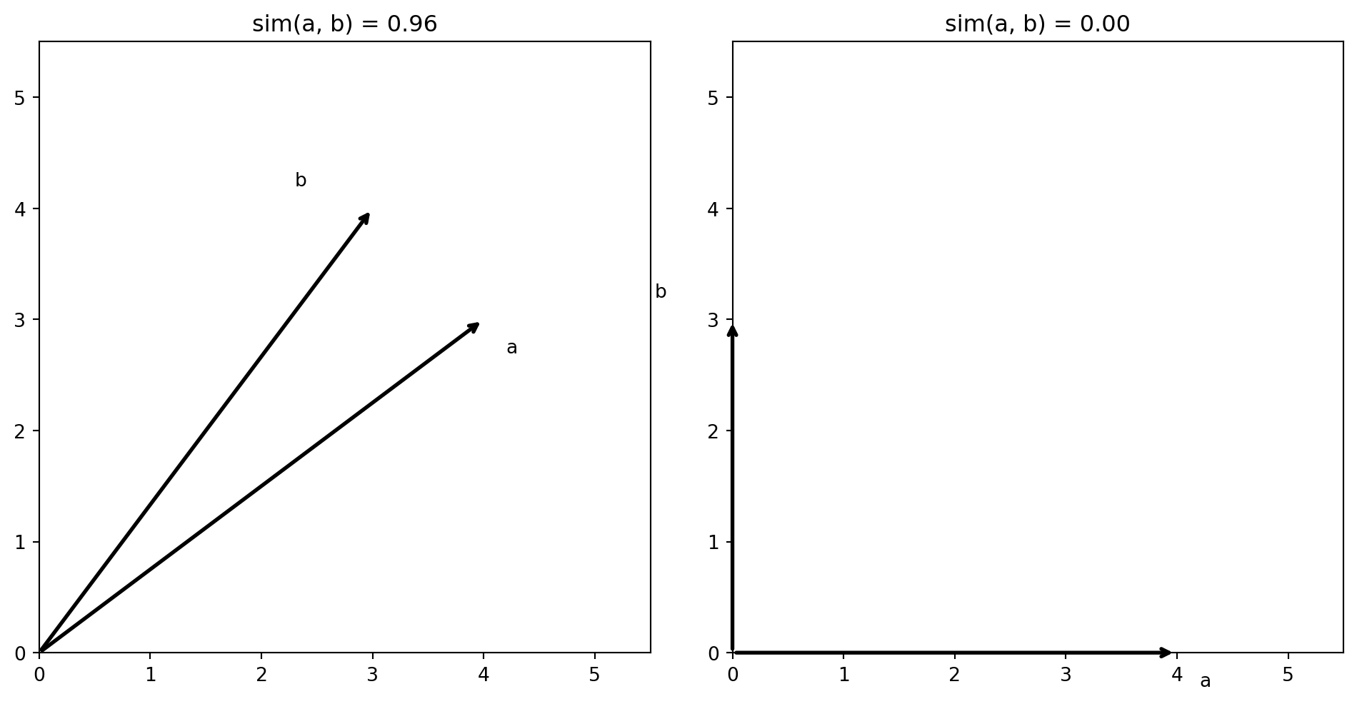
Before we move to embeddings, we need a way to measure how similar two vectors are. Recall from Lecture 1 that the dot product of two vectors \(\mathbf{a}\) and \(\mathbf{b}\) is:
The dot product is large when two vectors point in the same direction and zero when they are perpendicular. It is related to the angle \(\theta\) between the vectors by:
This ranges from \(-1\) (opposite directions) through \(0\) (perpendicular / no similarity) to \(+1\) (same direction / identical pattern). Normalizing by length is useful for text: a long article and a short article about the same topic will have high cosine similarity even though their raw word counts differ.
When \(\operatorname{sim}(\mathbf{a}, \mathbf{b}) = 0\), the vectors are orthogonal — they share nothing in common. In a BOW representation, two documents are orthogonal if they share no words at all. This is the core limitation we address next: in BOW space, “revenue” and “sales” are orthogonal even though they mean the same thing.
Cosine Similarity: A 2D Example
import numpy as npimport matplotlib.pyplot as pltfig, axes = plt.subplots(1, 2)# Left panel: two vectors pointing in similar directionsa1 = np.array([4, 3])b1 = np.array([3, 4])sim1 = np.dot(a1, b1) / (np.linalg.norm(a1) * np.linalg.norm(b1))ax = axes[0]ax.annotate("", xy=a1, xytext=(0, 0), arrowprops=dict(arrowstyle="->", lw=2))ax.annotate("", xy=b1, xytext=(0, 0), arrowprops=dict(arrowstyle="->", lw=2))ax.text(a1[0] +0.2, a1[1] -0.3, "a")ax.text(b1[0] -0.7, b1[1] +0.2, "b")ax.set_title(f"sim(a, b) = {sim1:.2f}")ax.set_xlim(0, 5.5)ax.set_ylim(0, 5.5)ax.set_aspect("equal")# Right panel: two perpendicular vectorsa2 = np.array([4, 0])b2 = np.array([0, 3])sim2 = np.dot(a2, b2) / (np.linalg.norm(a2) * np.linalg.norm(b2))ax = axes[1]ax.annotate("", xy=a2, xytext=(0, 0), arrowprops=dict(arrowstyle="->", lw=2))ax.annotate("", xy=b2, xytext=(0, 0), arrowprops=dict(arrowstyle="->", lw=2))ax.text(a2[0] +0.2, a2[1] -0.3, "a")ax.text(b2[0] -0.7, b2[1] +0.2, "b")ax.set_title(f"sim(a, b) = {sim2:.2f}")ax.set_xlim(0, 5.5)ax.set_ylim(0, 5.5)ax.set_aspect("equal")plt.tight_layout()plt.show()
Left: Two vectors pointing in nearly the same direction — high cosine similarity. Right: Two perpendicular vectors — zero cosine similarity, meaning they share nothing in common. In BOW space, two documents that use completely different words are orthogonal like this, even if they discuss the same topic using synonyms.
The Limits of Bag of Words
Every approach so far — BOW, TF-IDF, sentiment dictionaries, LDA — treats words as discrete symbols. Word \(j\) is a one-hot vector: all zeros except for a 1 in position \(j\). This means:
“Revenue” and “sales” are just as different as “revenue” and “giraffe” — both are orthogonal in the word-count space.
Synonyms get no credit for meaning the same thing.
The representation has no notion of semantic similarity.
We want a representation where words with similar meanings are close together in vector space. This is what word embeddings provide.
Word2Vec: Learning Word Vectors from Context
Mikolov et al. (2013) introduced Word2Vec, which learns a dense vector representation (an “embedding”) for each word from a large text corpus. The core idea:
“You shall know a word by the company it keeps.” — J.R. Firth (1957)
Words that appear in similar contexts should have similar embeddings. “Revenue” and “sales” often appear near the same words (“quarterly”, “growth”, “declined”), so their embeddings should be close.
Word2Vec uses a shallow neural network trained on a simple task: given a word, predict its surrounding context words (or vice versa). The learned weights of this network become the word embeddings.
Each word gets mapped to a dense vector, typically of dimension 100–300:
Compare this to the one-hot BOW vector for “revenue”, which is a sparse vector in \(\mathbb{R}^{50{,}000}\) with a single 1. The embedding is dramatically lower-dimensional and captures meaning.
Embeddings Capture Semantic Relationships
Word embeddings encode semantic relationships as geometric relationships in vector space. The most famous example:
where \(\mathbf{e}_{w_{dn}}\) is the embedding of the \(n\)-th word in document \(d\). This gives a dense, fixed-length vector for each document that can be fed into any downstream model (regression, classification, etc.).
Static vs. Contextual Embeddings
Word2Vec produces static embeddings: each word gets one vector, regardless of context. But many words have multiple meanings:
“The bank raised interest rates” (financial institution)
“We walked along the river bank” (edge of a river)
“I want to bank on this trade” (rely on)
In Word2Vec, all three uses of “bank” map to the same vector. This is a problem.
Contextual embeddings (ELMo, BERT, GPT) solve this by producing a different vector for each occurrence of a word, depending on the surrounding context. The vector for “bank” in “bank raised rates” is different from “bank” in “river bank.”
This is achieved by processing the entire sentence through a deep neural network (like the ones we saw in Lecture 9), so each word’s representation incorporates information from all the other words around it.
Part VII: Large Language Models
From Embeddings to LLMs
The progression of text representations mirrors the progression of ML models in this course — each step trades simplicity for expressiveness:
Representation
Dimension
Captures
Bag of words
\(V\) (~50,000)
Word presence
TF-IDF
\(V\) (~50,000)
Word importance
Word2Vec
~300
Semantic similarity
BERT / GPT
~768–1,024 per token
Context-dependent meaning
Large language models (LLMs) like BERT, GPT, and LLaMA take the contextual embedding idea to its extreme. They are massive neural networks — from 110 million parameters (BERT-base) to hundreds of billions (GPT-4) — pre-trained on enormous text corpora.
The key architectural innovation is the attention mechanism (Vaswani et al. 2017), which allows the model to weigh the relevance of every other word in a sentence when computing the representation of any given word. We will not cover the attention mechanism in detail, but the intuition matters: instead of processing text left-to-right, the model can “look at” the entire input simultaneously to resolve ambiguity.
The Attention Mechanism: Intuition
Consider two sentences:
“Swing the bat!”
“The bat flew at night.”
Traditional embeddings give “bat” the same vector in both sentences. The attention mechanism addresses this by computing context-dependent weights.
For each word, the model asks: “Which other words in this sentence are most relevant to understanding me?” The attention scores determine how much each surrounding word influences the representation:
In “Swing the bat” → high attention weight on “swing” → sports meaning
In “The bat flew at night” → high attention weight on “flew” and “night” → animal meaning
The result: “bat” gets a different vector in each sentence, one close to “baseball” and the other close to “animal.” This is what makes contextual embeddings so much more expressive than static ones.
Using LLMs for Finance
In practice, finance researchers use pre-trained LLMs in two ways:
1. Feature extraction (embeddings as inputs)
Pass a news article through a pre-trained model (e.g., BERT, RoBERTa) and extract the output embeddings. These dense vectors become features for a downstream model — logistic regression, Random Forest, neural network — that predicts returns, default, or sentiment.
This is how Chen, Kelly, and Xiu (2024) use LLMs to predict stock returns from news. They extract embeddings from several models and use them to construct long-short portfolios. Their best model (using RoBERTa embeddings) achieves an equal-weighted Sharpe ratio of 3.82, comparable to the SESTM approach but without requiring any feature engineering.
2. Zero-shot / few-shot classification
Ask the LLM directly: “Is this article positive or negative for the stock price?” Modern LLMs can perform sentiment classification without any training data, using only the prompt. This bypasses the entire pipeline of tokenization → TF-IDF → model fitting.
The trade-off: LLMs are computationally expensive, require significant hardware, and can behave unpredictably. Simpler methods like TF-IDF + logistic regression remain competitive for many tasks and are far easier to deploy and interpret.
The Full NLP Toolkit: Summary
We have covered a progression of methods, each building on the last:
Method
Type
What it does
Strengths
Weaknesses
BOW / TF-IDF
Representation
Count (or weight) words
Simple, interpretable, fast
Ignores word order and meaning
Sentiment dictionaries
Supervised (manual)
Score tone using word lists
Transparent, domain-specific
Rigid, misses context
SESTM
Supervised (learned)
Learn sentiment words from returns
Data-driven, high Sharpe
Requires labelled outcomes
LDA
Unsupervised
Discover latent topics
No labels needed, flexible
Hard to tune \(K\), slow
Word2Vec
Representation
Dense vectors from context
Captures meaning
Static, one vector per word
BERT / LLMs
Representation + model
Context-dependent embeddings
State of the art
Expensive, black box
For a class project or first pass at a research question, TF-IDF + a simple model (logistic regression, Lasso) is almost always the right starting point. Add complexity only when the simple approach fails.
Summary
What We Covered Today
Text as data: Financial text is abundant, forward-looking, and ultra-high dimensional. We worked with a corpus of WSJ articles to see the full pipeline in action.
Bag of words and TF-IDF: The simplest representations — word counts and importance-weighted counts. We built the term-document matrix and saw how TF-IDF downweights common words and highlights distinctive ones.
Sentiment analysis: Dictionary-based approaches (Loughran and McDonald 2011) classify words as positive/negative. Data-driven approaches like SESTM (Ke, Kelly, and Xiu 2019) learn which words carry sentiment from returns data.
Topic modeling: LDA (Blei, Ng, and Jordan 2003) discovers latent themes as mixtures of words, controlled by the Dirichlet distribution. Each document is a mixture of topics. Bybee et al. (2023) applied LDA to 800,000 WSJ articles and found that shifts in news attention predict macroeconomic variables.
Similarity and embeddings: Cosine similarity measures how closely two vectors point in the same direction. Word2Vec learns dense vectors where semantic similarity corresponds to geometric proximity. Contextual embeddings (BERT, GPT) produce different vectors for the same word depending on context.
LLMs: Massive pre-trained models used as feature extractors (Chen, Kelly, and Xiu 2024) or directly for zero-shot classification. Powerful but expensive and opaque. For most tasks, TF-IDF + a simple model is the right starting point.