Week 8: Nonlinear Classification
RSM338: Machine Learning in Finance
1 Introduction
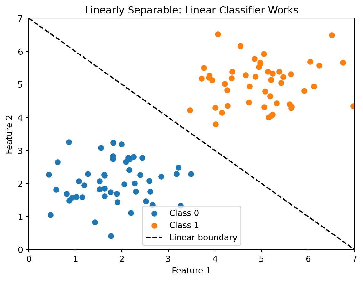
Last week we studied linear classifiers: logistic regression and LDA. Both methods draw a straight line (or hyperplane) through feature space to separate classes. This works well when classes are actually linearly separable — you can draw a straight line between them. But in many real-world applications, the boundary between classes isn’t linear, and linear classifiers will struggle.
Think about what “linearly separable” actually requires. For two features, it means we can draw a single straight line that perfectly divides the classes. For three features, a single flat plane. For \(p\) features, a single \((p-1)\)-dimensional hyperplane. That’s a strong assumption. It says that the combined effect of all features on the class label can be captured by a single linear combination \(w_0 + w_1 x_1 + \cdots + w_p x_p\), and the sign of that combination is all we need. In practice, the relationship between features and outcomes is often more complicated. Whether a loan defaults might depend on the interaction between credit score and debt-to-income ratio, not just their additive effects. A borrower with a 680 credit score and 20% DTI is very different from one with a 680 score and 45% DTI, and that distinction doesn’t reduce to a simple weighted sum.
Recall from Week 7 that logistic regression can handle nonlinear boundaries if we add the right transformed features (e.g., \(x_1^2\), \(x_1 x_2\)). The model stays linear in its parameters — we just give it richer inputs. But that approach has a big limitation: we have to know which transformations to use. With 2 features, adding squares and interactions is easy enough. With 50 features, there are 1,275 pairwise interactions and 50 squared terms — and we have no guarantee that quadratic terms are the right choice. Maybe the boundary depends on \(\log(x_3)\), or \(x_7 / x_{12}\), or some transformation we’d never think to try.
This is the feature engineering problem: the burden is entirely on us to figure out how to transform the raw inputs before handing them to a linear model. If we get the transformations right, the model works well. If we guess wrong, the model is systematically biased no matter how much data we have. And in most real applications, we simply don’t know the right transformations. Credit default depends on dozens of borrower characteristics in ways that no one fully understands — that’s precisely why we’re using machine learning in the first place.
We want methods that can learn nonlinear boundaries directly from the data, without us guessing the right feature transformations in advance. This chapter covers two such methods: k-Nearest Neighbors (k-NN) and Decision Trees. Both are nonparametric — they don’t assume a particular functional form for the decision boundary. Instead, they let the data itself determine the shape of the boundary. The flexibility comes at a cost — these methods are more prone to overfitting, especially with limited data — but they can discover patterns that linear models would miss entirely.
1.1 Parametric vs. Nonparametric Models
Before diving into the methods, it helps to understand the distinction between parametric and nonparametric models, because it explains both the power and the limitations of what we’re about to learn.
Parametric models like logistic regression assume the data follows a specific functional form. We estimate a fixed set of parameters (\(w_0, w_1, \ldots, w_p\)), and these parameters define the model completely. Once training is done, the training data can be thrown away — the model is fully captured by its parameters. This is both a strength and a weakness. The strength is efficiency: with \(n = 10{,}000\) observations, the model might have just \(p + 1 = 10\) parameters. All the information in those 10,000 observations is compressed into 10 numbers. This compression works beautifully when the assumed form is correct. But if the true relationship is nonlinear and we’ve assumed a linear form, no amount of data will fix the problem. The model is structurally incapable of capturing the pattern. This is the bias problem we discussed with underfitting in earlier weeks.
Nonparametric models make fewer assumptions about the functional form. Instead, they let the data determine the structure of the decision boundary. The model’s complexity can grow with the data — more data lets the model capture more detailed patterns. The tradeoff is that with limited data, these models are prone to overfitting. They have so much flexibility that they can memorize noise in the training set rather than learning genuine patterns. Managing this tradeoff — enough flexibility to capture real patterns, not so much that we fit noise — is the central challenge of nonparametric methods.
| Parametric | Nonparametric | |
|---|---|---|
| Structure | Fixed form (e.g., linear) | Flexible, data-driven |
| Parameters | Fixed number | Grows with data |
| Examples | Logistic regression, LDA | k-NN, Decision Trees |
| Risk | Bias if form is wrong | Overfitting with limited data |
Both k-NN and decision trees are nonparametric — they don’t assume a linear (or any particular) decision boundary. But they achieve flexibility in very different ways. k-NN uses the local structure of the data, making predictions based on nearby observations. Decision trees partition the feature space into regions using simple rules. Understanding both gives us a sense of the range of strategies available for nonlinear classification.
To ground the discussion, consider a bank deciding whether to approve a loan. The outcome is binary: the borrower either repays in full (class 0) or defaults (class 1). Based on features like credit score, income, and debt-to-income ratio, can we predict who will default? The relationship between features and default is rarely linear. A borrower with moderate income and moderate credit score might default, while someone with either very high income OR very high credit score might not — this creates complex, nonlinear boundaries. A linear model would have to pick one dividing line and live with it; the methods in this chapter can adapt to these more complex patterns.
2 k-Nearest Neighbors
2.1 The Idea
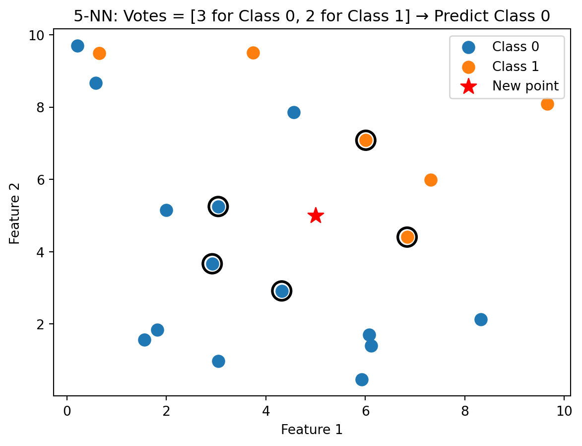
k-Nearest Neighbors (k-NN) is based on a simple idea: similar observations should have similar outcomes. To classify a new observation, we find the \(k\) training observations closest to it, take a vote among those \(k\) neighbours, and assign the majority class. If you want to know whether a new loan applicant will default, look at applicants in the training data who are most similar to them. If most of those similar applicants defaulted, predict default.
The underlying assumption is one of smoothness: observations that are close together in feature space should tend to have the same class label. This is a weaker assumption than the parametric models make. We’re not saying the boundary is a line, or a parabola, or any particular shape. We’re just saying that the class label doesn’t change abruptly as you move through feature space — nearby points tend to behave similarly. This is often reasonable. A borrower with a 720 credit score and 25% DTI is probably similar in default risk to a borrower with a 715 credit score and 26% DTI. The smoothness assumption is what lets k-NN generalize from training data to new observations.
No training phase is needed — k-NN stores all the training data and does the work at prediction time. This is sometimes called a “lazy learner” because it defers all computation to the prediction step. Every other model we’ve studied (linear regression, logistic regression, LDA) has a training phase where we estimate parameters, and a separate prediction phase where we plug new observations into the learned model. k-NN skips the first step entirely. It just memorizes the training data and does all the work when you ask it to make a prediction. This has implications for computational cost: training is instant (just save the data), but prediction is expensive (you have to compare the new point to every stored training point).
2.2 Distance
k-NN needs to measure how “close” two observations are. This is the same distance concept we used in clustering (Week 4). For two observations \(\mathbf{x}_i\) and \(\mathbf{x}_j\) with \(p\) features, we use Euclidean distance:
\[d(\mathbf{x}_i, \mathbf{x}_j) = \|\mathbf{x}_i - \mathbf{x}_j\| = \sqrt{\sum_{k=1}^{p} (x_{ik} - x_{jk})^2}\]
This is just the Pythagorean theorem generalized to \(p\) dimensions. In two dimensions it’s the straight-line distance you’d measure with a ruler. In higher dimensions it works the same way — square each difference, sum them up, take the square root.
Two reminders from Week 4. First, always standardize features before computing distances. Features on different scales will make the distance dominated by whichever feature has the largest numbers. Suppose we have two features: annual income (ranging from $30,000 to $200,000) and DTI ratio (ranging from 0.10 to 0.60). The income feature varies by hundreds of thousands while DTI varies by fractions. Without standardization, the Euclidean distance between any two borrowers will be almost entirely determined by their income difference — the DTI difference is negligible by comparison. This means the “nearest neighbours” are really just the neighbours with the most similar income, regardless of their DTI. Standardizing each feature to mean 0 and standard deviation 1 puts them on equal footing.
Second, distance is the norm of a difference vector. The \(L_2\) (Euclidean) norm is the default choice in k-NN. Manhattan distance (\(L_1\)) is an alternative that sums absolute differences rather than squared differences, making it less sensitive to outliers in individual features. In practice, the choice of distance metric rarely matters as much as feature scaling and the choice of \(k\).
2.3 The Algorithm
More formally, the k-NN algorithm works as follows. Given training data \(\{(\mathbf{x}_1, y_1), \ldots, (\mathbf{x}_n, y_n)\}\), a new point \(\mathbf{x}\), and the number of neighbours \(k\):
- Compute the distance from \(\mathbf{x}\) to every training observation \(\mathbf{x}_i\)
- Identify the \(k\) training observations with the smallest distances — call this set \(\mathcal{N}_k(\mathbf{x})\)
- Assign the class that appears most frequently among the \(k\) neighbours:
\[\hat{y} = \arg\max_c \sum_{i \in \mathcal{N}_k(\mathbf{x})} \ind_{\{y_i = c\}}\]
The notation \(\ind_{\{y_i = c\}}\) is the indicator function: it equals 1 if \(y_i = c\) and 0 otherwise. So we’re just counting votes. The \(\arg\max_c\) notation means “find the class \(c\) that maximizes the count.” If 3 out of 5 neighbours are class 0 and 2 are class 1, the count is higher for class 0, so we predict class 0.
With \(k = 1\), we classify based on the single closest training point — the new observation inherits the class of its nearest neighbour. With \(k = 5\), we take a majority vote among the 5 nearest neighbours, which is more robust to noise. A single neighbour could be a noisy outlier, but it’s less likely that 3 out of 5 neighbours are all outliers.
Notice that k-NN can also produce class probabilities, not just hard class predictions. Instead of taking the majority vote, we can report the fraction of neighbours in each class. If 4 out of 5 neighbours are class 1, we can say \(\hat{P}(y = 1) = 4/5 = 0.8\). This is useful when we need probability estimates — for example, to compute AUC or to set a custom classification threshold. The probability estimates from k-NN tend to be coarser than those from logistic regression (they can only take values that are multiples of \(1/k\)), but they’re still informative.
Step 1 is where the computational cost comes in. For every new observation we want to classify, we must compute the distance to all \(n\) training observations. If the training set is large (say \(n = 100{,}000\)), this means 100,000 distance computations per prediction. For real-time applications like fraud detection, where predictions need to happen in milliseconds, this can be a serious bottleneck.
2.4 Decision Boundaries
Unlike linear classifiers, k-NN doesn’t produce an explicit formula for the decision boundary. There’s no equation you can write down that describes where the boundary is. Instead, the boundary is implicit — it’s defined by the training data. To find the boundary, you’d have to classify a dense grid of points across the feature space and see where the predicted class changes. We can visualize what this looks like by doing exactly that: classifying every point in a grid and colouring the regions by predicted class.
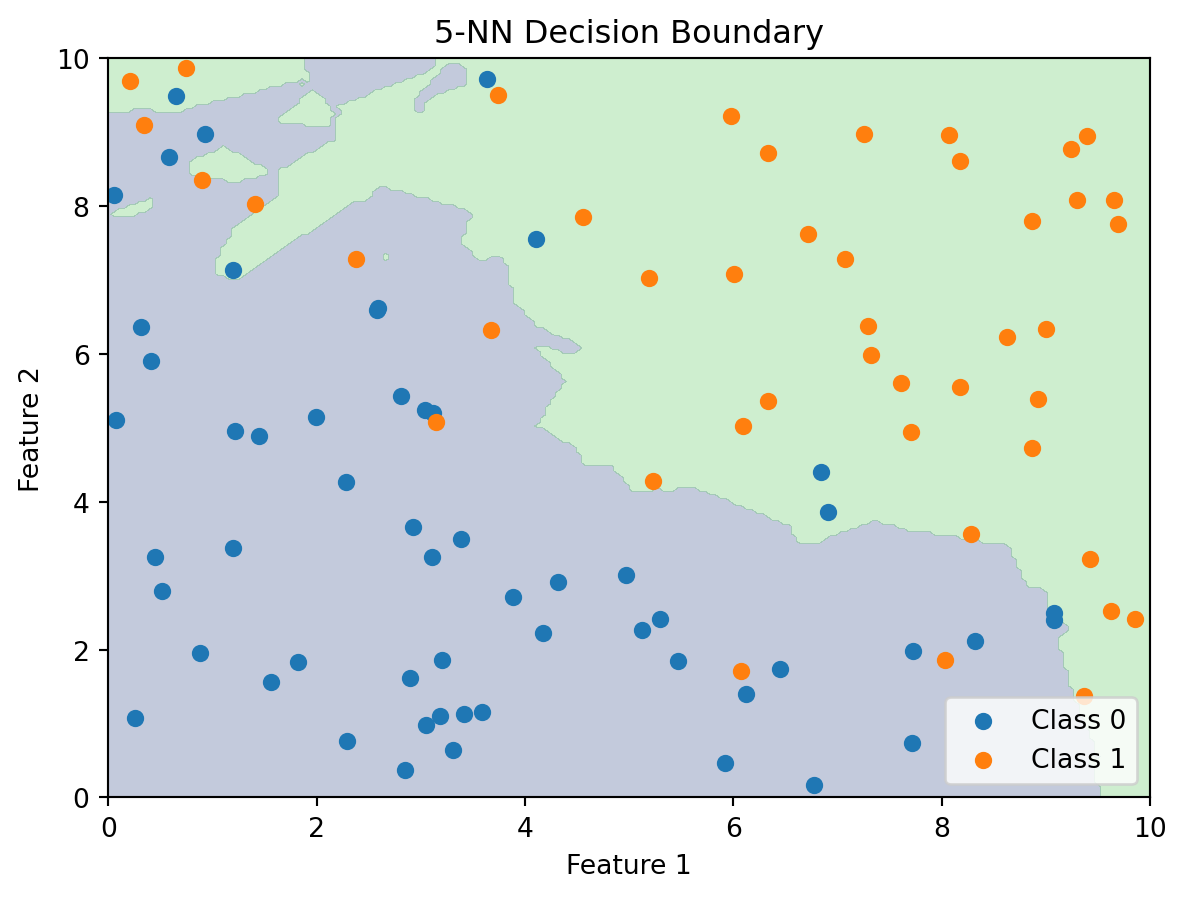
The k-NN decision boundary is nonlinear and adapts to the local density of the data. Where there are many class 0 observations clustered together, the boundary curves around them to create a class 0 region. Where class 1 observations dominate, the boundary expands to accommodate them. The boundary naturally forms complex shapes without us specifying any functional form — no quadratic terms, no interaction terms, no feature engineering at all.
For \(k = 1\), the decision boundary is especially interesting. Each training point “owns” the region of feature space closest to it. The result is a Voronoi tessellation — the space is partitioned into polygonal cells, one per training point, where every point in a cell is closest to the training point at its centre. The predicted class in each cell is simply the class of the training point that owns it. As \(k\) increases, these sharp boundaries get smoothed out because multiple neighbours contribute to each prediction.
2.5 Choosing k: The Bias-Variance Tradeoff
The choice of \(k\) controls the bias-variance tradeoff, and understanding the two extremes makes the tradeoff concrete.
With \(k = 1\), the model memorizes the training data perfectly. Every training observation is its own nearest neighbour, so the model always predicts the correct class for training points. Training accuracy is 100% — but this is misleading. The model is also memorizing noise. If a single training point has been mislabelled (or is just an unusual observation), the model will carve out a region of feature space around it and make the wrong prediction for any new point that falls nearby. This is high variance: the decision boundary is jagged and erratic, changing dramatically if we add or remove a single training point.
With \(k = n\) (the entire training set), every prediction is the same: the majority class in the training data. If 80% of training observations are class 0, the model predicts class 0 for everything, regardless of the features. The decision boundary doesn’t exist — the entire space is assigned to one class. This is high bias: the model has so little flexibility that it ignores all the information in the features. It’s essentially just predicting the base rate.
Between these extremes, we’re trading off flexibility against stability. Small \(k\) gives a boundary that closely follows the training data, capturing complex local patterns but also fitting noise. Large \(k\) gives a smoother boundary that’s more robust to individual noisy points but can miss genuine local structure. The boundary smooths out as \(k\) increases because each prediction averages over more neighbours, and averaging reduces variance.
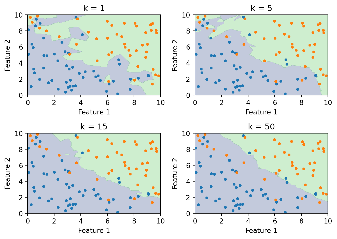
As \(k\) increases, the boundary becomes smoother. With \(k = 1\), every training point gets its own jagged region. With large \(k\), the boundary approaches the overall majority class and eventually becomes trivial.
We choose \(k\) using cross-validation, just as we chose regularization parameters in earlier weeks. Split the training data into folds, evaluate each candidate \(k\), and pick the one that maximizes cross-validated performance. The cross-validation procedure is the same one we used for ridge and lasso regression (Week 5) — nothing new here, just a different hyperparameter being tuned.
A common heuristic is to try odd values of \(k\) (to avoid ties in binary classification) up to around \(\sqrt{n}\). But cross-validation is more reliable than any rule of thumb because the right \(k\) depends on the data — how noisy it is, how complex the true boundary is, and how many observations are available.
from sklearn.neighbors import KNeighborsClassifier
from sklearn.model_selection import cross_val_score
import numpy as np

# Try different values of k
k_values = range(1, 31)
cv_scores = []

for k in k_values:
    knn = KNeighborsClassifier(n_neighbors=k)
    scores = cross_val_score(knn, X_train, y_train, cv=5)
    cv_scores.append(scores.mean())

best_k = k_values[np.argmax(cv_scores)]
print(f"Best k: {best_k} with CV accuracy: {max(cv_scores):.3f}")
Best k: 19 with CV accuracy: 0.8502.6 Advantages and Disadvantages
k-NN has several attractive properties. It’s simple to understand and implement — there’s no optimization algorithm, no loss function, no iterative training procedure. It naturally handles multi-class problems (just take a vote among more than two classes). It can capture arbitrarily complex nonlinear boundaries without any assumptions about the data distribution. And it makes no assumptions about the functional form of the decision boundary, so it can’t be “wrong” in the way a linear model can be wrong.
On the other hand, k-NN has real limitations. Prediction is slow because classifying a single new point requires computing the distance to every training observation. It requires careful feature scaling (as discussed above). And it’s sensitive to irrelevant features: since all features contribute equally to distance, adding features that are unrelated to the class label dilutes the signal from the useful features. Unlike logistic regression, where an irrelevant feature would just get a coefficient near zero, k-NN has no mechanism to ignore features — they all go into the distance calculation with equal weight.
2.7 The Curse of Dimensionality
The most fundamental limitation of k-NN is the curse of dimensionality. k-NN relies on distance, and distance breaks down in high dimensions. This isn’t just a theoretical concern — it’s the reason k-NN is rarely used with more than 20 or so features. There are three related problems.
First, the space becomes sparse. Think about what happens as we add dimensions. In one dimension, 100 points spread along a line cover it reasonably well. In two dimensions, the same 100 points are scattered across a square — much more space to fill. In three dimensions, they’re floating in a cube. By the time we reach 50 dimensions, those 100 points are lost in a 50-dimensional hypercube. The volume of the space grows exponentially with the number of dimensions, so the amount of data we need to “fill” the space grows exponentially too. To get the same density of points in 50 dimensions that 100 points give us in 1 dimension, we’d need \(100^{50}\) points — a number far larger than the number of atoms in the universe.
Second, you need more data to have local neighbours. The whole premise of k-NN is that we can find training observations that are “close” to the new point. But if the space is mostly empty, the \(k\) “nearest” neighbours may actually be quite far away. In high dimensions, even the closest training point might be in a very different part of the feature space. And if the neighbours aren’t truly local, their class labels aren’t informative about the new point. The smoothness assumption — nearby points have similar labels — only helps if “nearby” actually means nearby.
Third, distances become less informative. Euclidean distance sums \(p\) squared differences, one per feature. As \(p\) grows, each observation’s distance to every other observation converges to roughly the same value — a consequence of the law of large numbers. When the number of features is large, the ratio of the farthest distance to the nearest distance approaches 1. In other words, every point is approximately equidistant from every other point. The concept of “nearest neighbour” becomes meaningless because there’s no meaningful difference between the nearest and farthest neighbours.
These three problems are all manifestations of the same underlying issue: in high dimensions, the data is too spread out for local methods to work. This is why k-NN is best suited for problems with a moderate number of features (perhaps \(p < 20\), depending on the sample size). For high-dimensional problems, methods that can effectively ignore irrelevant features — like regularized logistic regression or the tree-based methods we’ll study next — tend to perform much better.
3 Decision Trees
3.1 The Intuition
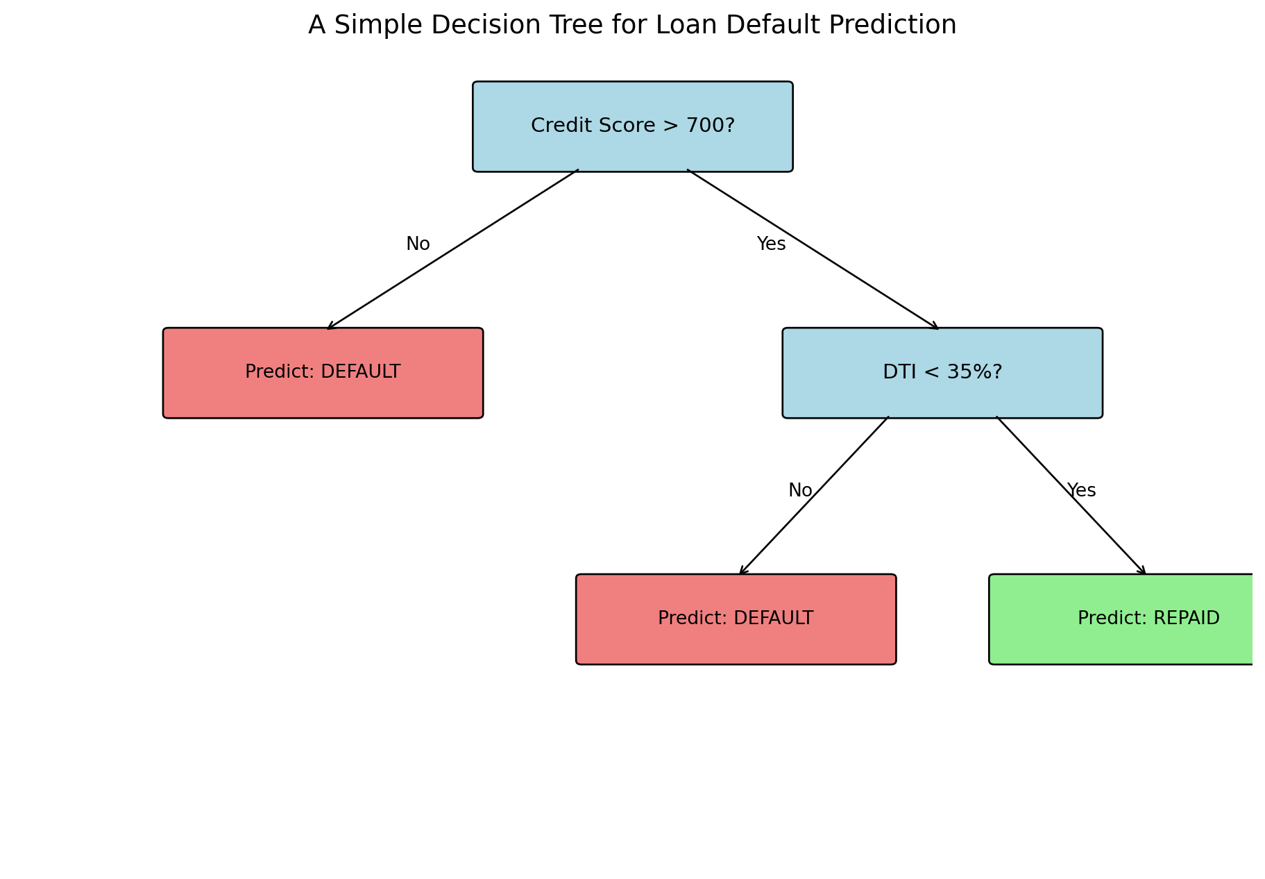
Decision trees mimic how humans make decisions: a series of yes/no questions. Consider a loan officer evaluating an application. First question: is the credit score above 700? If no, deny the loan (high risk). If yes, continue to the next question: is the debt-to-income ratio below 35%? If no, deny (medium risk). If yes, approve (low risk).
This is a very natural way to think about classification. Humans already make decisions this way — we just don’t usually formalize it. A doctor diagnosing a patient asks a sequence of questions, each narrowing down the possibilities. An investor screening stocks might first filter by market cap, then by P/E ratio, then by dividend yield. Each question splits the population into subgroups, and the subgroups get progressively more homogeneous.
Decision trees automate this process — they learn which questions to ask and in what order, choosing the questions that best separate the classes at each step. The result is a flowchart-like structure that anyone can follow, making decision trees one of the most interpretable models in machine learning. A bank regulator can look at a decision tree and understand exactly why a particular loan was approved or denied, which is much harder with a logistic regression model (where the decision depends on the combined effect of all features) and essentially impossible with k-NN (where the decision depends on the specific training points that happened to be nearby).
A tree has three types of components. The root node is the first split at the top of the tree — the first question we ask. Internal nodes are decision points that split the data further based on additional questions. Leaf nodes (also called terminal nodes) are where predictions happen — once we reach a leaf, we stop asking questions and output a class prediction. The depth of a tree is the number of splits from root to leaf along the longest path. A depth-1 tree (called a “stump”) asks just one question; a depth-3 tree asks up to three sequential questions before making a prediction.
Every observation that arrives at a leaf gets the same prediction: the majority class among the training observations that ended up in that leaf. So a tree with 8 leaves divides the entire population into 8 groups, each with a single class prediction. The tree’s “model” is just a lookup table: which group does this observation belong to, and what’s the prediction for that group?
3.2 How Trees Partition the Feature Space
Each split in a decision tree divides the feature space with an axis-aligned boundary — a line parallel to one of the coordinate axes. “Axis-aligned” means the split uses only one feature at a time: “is credit score above 700?” rather than “is credit score plus twice the income above some threshold.” This is different from linear classifiers, which can use arbitrary linear combinations of features for the boundary. The tree creates rectangular regions, and each leaf corresponds to one region. All observations in that region get the same prediction.
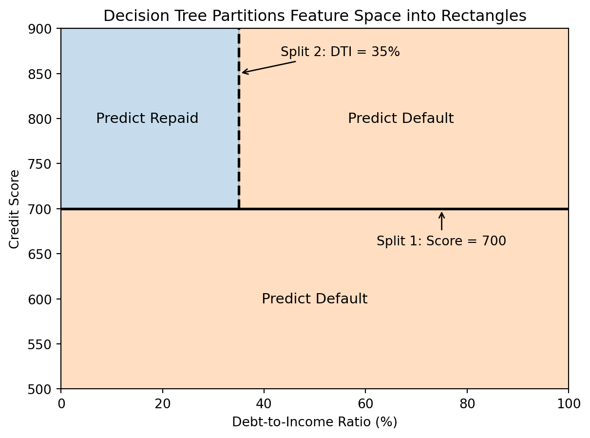
This is a limitation compared to k-NN’s curved boundaries — trees can only make axis-aligned cuts. If the true decision boundary is a diagonal line (say, “default if credit score minus twice the DTI is below some threshold”), a tree would need many small rectangular cuts to approximate it, like building a staircase to approximate a slope. But the axis-aligned constraint is also what makes trees so interpretable: each split is a simple, human-readable rule like “credit score > 700.” You can explain a tree’s prediction to a non-technical audience, which is rarely true for other nonlinear models.
3.3 Recursive Partitioning and Impurity
Decision trees are built by greedy, recursive partitioning. The algorithm starts with all training data at the root. It considers every possible split — every feature and every threshold for that feature — and picks the one that best separates the classes. It then splits the data into two groups based on this rule and recursively applies the same process to each group. It stops when a stopping criterion is met (e.g., minimum samples per leaf, maximum depth, or no further improvement possible).
The word “greedy” is important. The algorithm makes the best decision at each step without looking ahead. It doesn’t consider whether a seemingly bad split now might lead to great splits later. This is a deliberate simplification. Finding the globally optimal tree — the one that makes the best possible predictions overall — is computationally intractable (it’s an NP-hard problem). The number of possible trees grows astronomically with the number of features and observations. The greedy approach doesn’t guarantee the best tree, but it produces a good tree quickly.
The word “recursive” means the same algorithm is applied repeatedly. After the first split creates two child nodes, we apply the same splitting procedure to each child independently. The left child picks its own best split, the right child picks its own. Then each of their children picks a split, and so on, until we stop. This recursive structure is what creates the tree.
The key question is: how do we define “best” split? A good split should create child nodes that are more “pure” than the parent — ideally, each child contains only one class. We measure impurity, which quantifies how mixed the classes are in a node. A pure node (all one class) has impurity = 0. A maximally impure node (50/50 split between classes) has the highest impurity. We want splits that reduce impurity as much as possible.
For a node with \(n\) observations where \(p_c\) is the proportion belonging to class \(c\), the two most common impurity measures are:
Gini impurity: \[\text{Gini} = 1 - \sum_c p_c^2\]
Entropy: \[\text{Entropy} = -\sum_c p_c \log_2(p_c)\]
Both measures equal 0 for a pure node and are maximized when classes are equally mixed. For binary classification with \(p\) being the proportion in class 1, Gini simplifies to \(2p(1-p)\).
To build intuition, consider a node where 90% of observations are class 0 and 10% are class 1. This node is already fairly pure — it’s mostly class 0. Gini impurity is \(1 - 0.9^2 - 0.1^2 = 0.18\), which is low. Now consider a node where the split is 50/50. This is the most uncertain we can be. Gini is \(1 - 0.5^2 - 0.5^2 = 0.5\), the maximum. If we can find a split that turns this 50/50 node into two children that are 90/10 and 10/90, we’ve reduced impurity substantially.
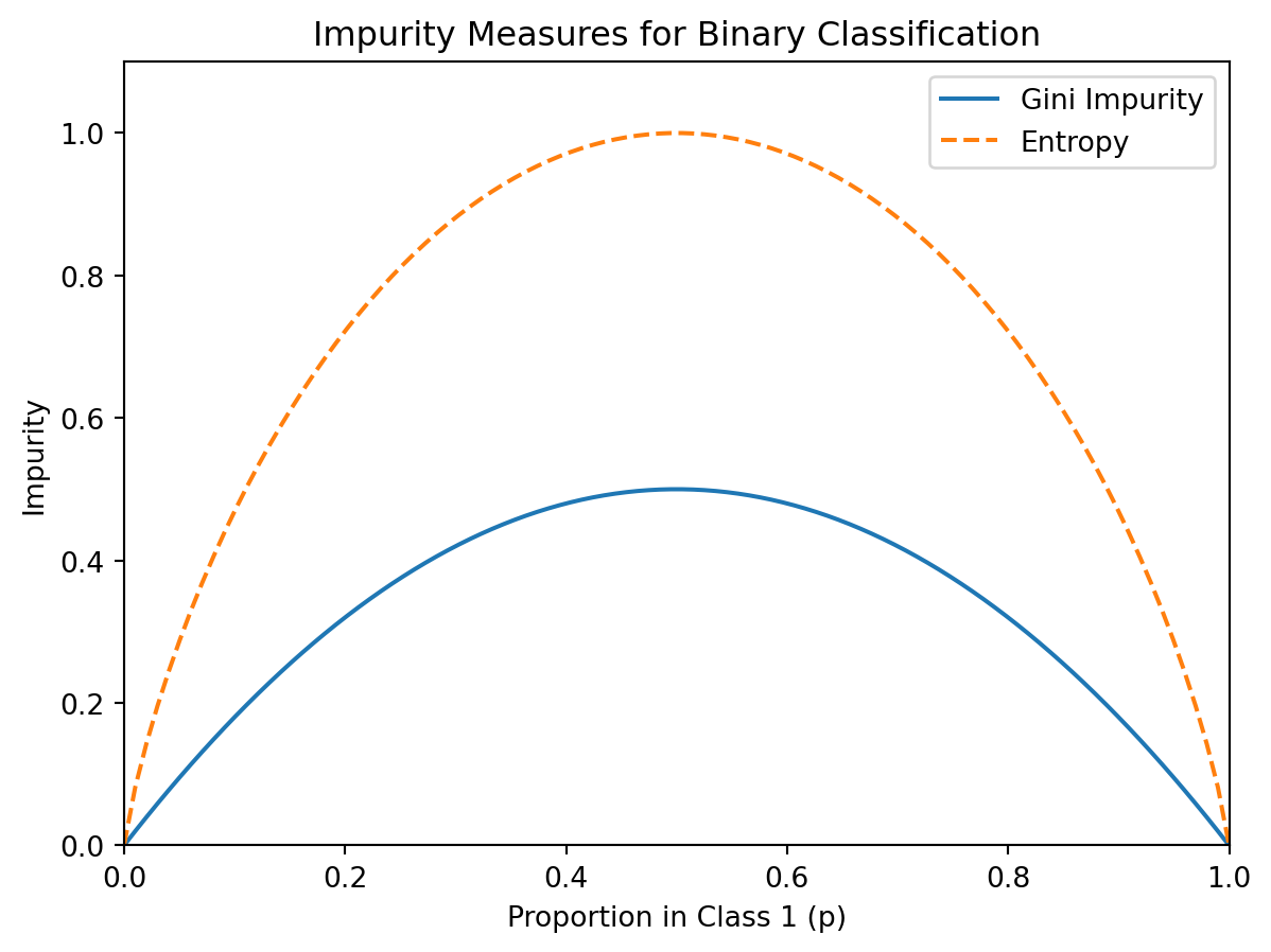
Both measures are minimized (= 0) when \(p = 0\) or \(p = 1\) (pure node) and maximized when \(p = 0.5\) (maximum uncertainty). Entropy is measured in “bits” (because of the \(\log_2\)), which connects to information theory — a 50/50 split requires 1 bit of information to resolve, while a 90/10 split requires much less. In practice, Gini and entropy produce very similar trees. Gini impurity is the default in scikit-learn and is slightly faster to compute (no logarithm needed).
3.4 Information Gain
Information gain measures how much a split reduces impurity. If a parent node \(P\) is split into children \(L\) (left) and \(R\) (right):
\[\text{Information Gain} = \text{Impurity}(P) - \left[\frac{n_L}{n_P} \cdot \text{Impurity}(L) + \frac{n_R}{n_P} \cdot \text{Impurity}(R)\right]\]
where \(n_P\), \(n_L\), \(n_R\) are the number of observations in the parent, left child, and right child. The term in brackets is the weighted average impurity of the children, weighted by how many observations go to each side. The weighting matters: a split that sends 99 observations to one child and 1 to the other is less informative than a split that divides the data more evenly, even if the single-observation child is perfectly pure. The best split is the one that maximizes information gain — the biggest drop from parent impurity to the weighted average child impurity.
As a concrete example, suppose we have 100 loan applicants: 60 repaid, 40 defaulted. The parent Gini impurity is \(1 - (0.6)^2 - (0.4)^2 = 0.48\). If we split on credit score > 700, we get a left child (below 700) with 30 observations (10 repaid, 20 default) giving Gini = 0.444, and a right child (above 700) with 70 observations (50 repaid, 20 default) giving Gini = 0.408. The information gain is \(0.48 - [0.3 \times 0.444 + 0.7 \times 0.408] = 0.061\). We’d compute this for all possible features and thresholds, then choose the split with highest gain.
The greedy algorithm tries every possible split at each node. For a continuous feature like credit score, this means considering every unique value as a potential threshold. If there are \(n\) unique values, we evaluate up to \(n-1\) possible splits for that feature. For a categorical feature like home ownership (own, mortgage, rent), we consider groupings of the categories into two sets. The algorithm evaluates all of these, for every feature, and picks the single best split. This brute-force search sounds expensive, but it’s actually efficient because the observations can be sorted by each feature once, and then class counts can be updated incrementally as we slide the threshold through the sorted values.
3.5 Building and Visualizing Trees in Python
Let’s see how decision trees work in practice. We’ll generate some synthetic data where default probability depends on both credit score and DTI through a nonlinear relationship (using a logistic function), then fit a tree and examine what it learns.
from sklearn.tree import DecisionTreeClassifier
import numpy as np

# Generate sample data
np.random.seed(42)
n = 200
credit_score = np.random.normal(700, 50, n)
dti = np.random.normal(30, 10, n)
X = np.column_stack([credit_score, dti])

# Default probability depends on both features
prob_default = 1 / (1 + np.exp(0.02 * (credit_score - 680) - 0.05 * (dti - 35)))
y = (np.random.random(n) < prob_default).astype(int)

# Fit decision tree
tree = DecisionTreeClassifier(max_depth=3, random_state=42)
tree.fit(X, y)

print(f"Tree depth: {tree.get_depth()}")
print(f"Number of leaves: {tree.get_n_leaves()}")
print(f"Training accuracy: {tree.score(X, y):.3f}")
Tree depth: 3
Number of leaves: 8
Training accuracy: 0.720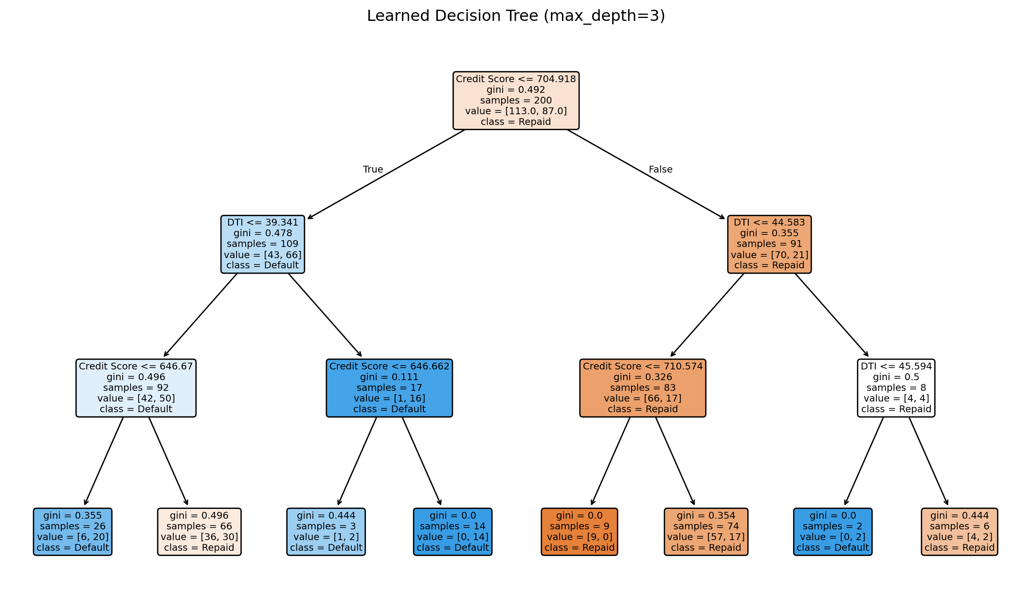
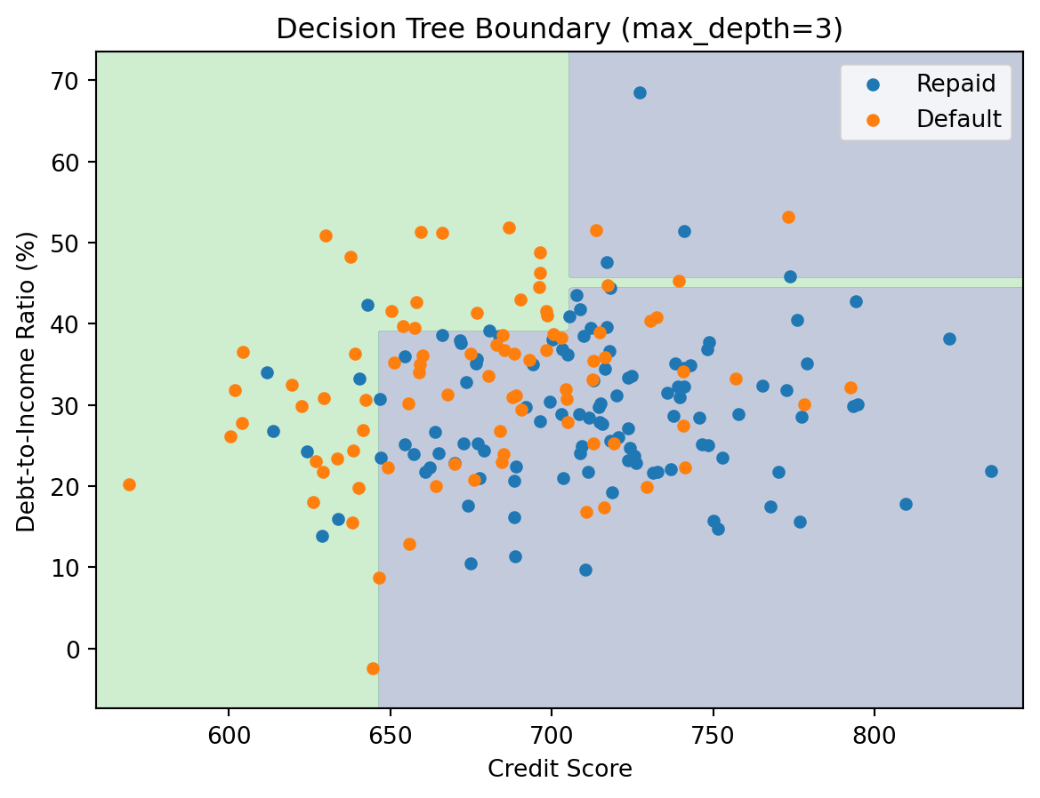
The tree learns splits automatically from the data. Each node in the visualization shows the split condition (e.g., “Credit Score <= 703.5”), the Gini impurity at that node, the number of samples that reached it, and the class distribution (how many in each class). The colour of each node reflects the majority class — bluer for “Repaid,” oranger for “Default.” Darker colours indicate higher purity. You can trace any path from root to leaf to understand exactly why the tree makes a particular prediction.
We can also visualize the decision boundary in feature space. Since each split is a horizontal or vertical line (axis-aligned), the resulting regions are always rectangles.
3.6 Controlling Tree Complexity
A fully grown decision tree can memorize the training data perfectly — just keep splitting until every leaf contains observations from a single class. With enough depth, you can always achieve 100% training accuracy. But this is almost always overfitting. The tree has carved the feature space into tiny regions, each tailored to the specific training observations that happened to land there. A new observation that falls in one of these tiny regions gets a prediction based on perhaps 2 or 3 training points, which is unreliable.
There are two strategies to prevent overfitting. Pre-pruning (also called early stopping) prevents the tree from growing too complex in the first place. We set constraints during the growing process: max_depth limits the number of levels in the tree, min_samples_split requires a node to have at least some minimum number of observations before we’ll consider splitting it, and min_samples_leaf requires each child to have at least some minimum number of observations after a split. Any of these will stop the tree from growing too deep and creating those tiny, unreliable leaf nodes.
Post-pruning takes the opposite approach: grow the full tree first, then prune it back. The idea is that some branches of the tree improve training accuracy but not test accuracy — they’re fitting noise. Post-pruning removes these branches. In scikit-learn, this is controlled by the ccp_alpha parameter (cost-complexity pruning), which penalizes trees for having too many leaves. A larger ccp_alpha produces a more aggressive prune and a smaller tree.
In either case, the hyperparameters (max_depth, min_samples_leaf, ccp_alpha) are chosen via cross-validation, just like \(k\) in k-NN or \(\lambda\) in ridge/lasso regression. The pattern is always the same: there’s a knob that controls model complexity, and we use cross-validation to find the setting that generalizes best.
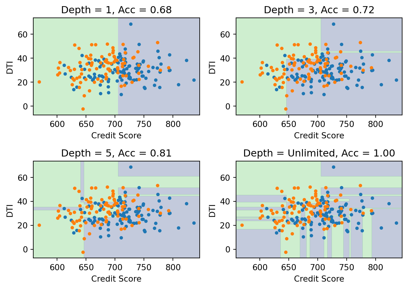
Deeper trees create more complex boundaries. With unlimited depth, the tree can achieve 100% training accuracy, but the boundary becomes so jagged and fragmented that it’s clearly fitting noise rather than learning a genuine pattern. The depth-3 tree captures the broad structure — credit score and DTI matter in roughly the way we’d expect — while the unlimited tree creates dozens of tiny regions that have no interpretable meaning.
3.7 Advantages and Disadvantages
Decision trees have several appealing properties. They are easy to interpret and explain — you can print the tree and walk through the decision rules with a non-technical audience. This “white-box” property is valuable in regulated industries like banking, where model decisions may need to be justified to regulators or customers. Trees handle both numeric and categorical features without any special encoding. They require no feature scaling (since each split uses only one feature at a time, the scale of other features is irrelevant). They naturally capture interactions between features: if the effect of DTI on default depends on credit score, a tree can discover this by splitting on credit score first and then splitting differently on DTI in each branch. And once the tree is built, prediction is fast — just walk from root to leaf, making one comparison at each node.
On the downside, trees can only produce axis-aligned boundaries, which means they need many splits to approximate diagonal or curved boundaries. They have high variance: small changes in the training data can produce a completely different tree. If the top split changes (because a slightly different training set would have chosen a different feature), the entire structure below it changes too. They’re prone to overfitting without regularization, and the greedy splitting algorithm may not find the globally optimal tree.
The high variance problem is arguably the biggest practical limitation of decision trees. A single tree is unstable — but averaging many trees together can be extremely powerful. This is the idea behind ensemble methods (Random Forests, Gradient Boosting), which we’ll cover in Week 9. Ensembles use individual trees as building blocks and combine them in ways that dramatically reduce variance while retaining flexibility.
4 Comparing k-NN and Decision Trees
Neither method dominates — the best choice depends on the data and the application requirements. The table below summarizes the tradeoffs.
| Aspect | k-NN | Decision Trees |
|---|---|---|
| Decision boundary | Flexible, curved | Axis-aligned rectangles |
| Training | None (stores data) | Builds tree structure |
| Prediction speed | Slow (compare to all training) | Fast (traverse tree) |
| Interpretability | Low (black-box) | High (rules) |
| Feature scaling | Required | Not required |
| High dimensions | Struggles (curse of dim.) | Handles better |
| Missing data | Problematic | Can handle |
The two methods have complementary strengths. k-NN produces smooth, curved boundaries that can conform to any shape, but it treats all features equally and breaks down in high dimensions. Decision trees produce blocky, axis-aligned boundaries that need many splits to approximate curves, but they can effectively ignore irrelevant features (they simply won’t split on them) and scale better to high-dimensional data.
k-NN is a good choice when you have low to moderate dimensionality (say \(p < 20\)), the decision boundary is expected to be complex and curved, interpretability is not critical, and the data is relatively dense. In finance, k-NN appears in anomaly detection (fraudulent transactions look different from neighbours in feature space), collaborative filtering (recommend assets held by similar investors), and pattern matching (find historical periods with similar market conditions to the current environment).
Decision trees are a good choice when interpretability is important (need to explain decisions), you have mixed feature types (numeric and categorical together), there may be complex interactions between features, fast prediction is required, or you plan to use them as building blocks for ensembles. In finance, decision trees appear in credit scoring (regulators may require that lending decisions be explainable), customer segmentation (which groups of clients have similar needs?), and risk management (clear rules for categorizing exposures).
In practice, individual decision trees are rarely used on their own for high-stakes predictions because of their high variance. But they’re the foundation of ensemble methods like Random Forests and Gradient Boosting, which are among the most competitive models in applied machine learning. k-NN, meanwhile, is rarely the top performer on structured tabular data but remains valuable in specialized applications where the notion of “similarity” is central to the problem.
5 Application: Lending Club Data
5.1 The Dataset
Lending Club was a peer-to-peer lending platform that operated from 2007 to 2020, where individuals could lend money to other individuals. Unlike a traditional bank, where a single institution makes all the lending decisions, Lending Club connected individual investors with individual borrowers. Investors could browse loan applications, see borrower characteristics, and decide which loans to fund.
The classification problem is: given borrower characteristics at the time of application, predict whether the loan will be repaid or will default. Features include FICO score (a credit score ranging from 300 to 850 that summarizes a borrower’s credit history), annual income, debt-to-income ratio (total monthly debt payments divided by monthly income), and home ownership status. This is a real business problem with significant financial stakes — approving a bad loan costs money (the lender loses the principal), but rejecting a good loan loses revenue (the lender misses out on interest income). The dataset we use was compiled by John Hull for his machine learning textbook, with a pre-split into training and test sets.
import pandas as pd

# Load Lending Club data (pre-split by Hull)
train_data = pd.read_excel('../Slides/lendingclub_traindata.xlsx')
test_data = pd.read_excel('../Slides/lendingclub_testdata.xlsx')

# Check columns and target
print(f"Training samples: {len(train_data)}")
print(f"Test samples: {len(test_data)}")
print(f"\nTarget distribution in training data:")
print(train_data['loan_status'].value_counts(normalize=True))
Training samples: 8695
Test samples: 5916
Target distribution in training data:
loan_status
1 0.827602
0 0.172398
Name: proportion, dtype: float64The data is imbalanced: most loans are repaid. This is realistic — a lending platform wouldn’t survive if most loans defaulted. But imbalanced data creates a subtle problem for model evaluation. If 80% of loans are repaid, a model that predicts “repaid” for every single application — ignoring the features entirely — achieves 80% accuracy. That sounds good, but the model is completely useless: it would never flag a single default. This is why we use AUC (area under the ROC curve) rather than accuracy as our evaluation metric. AUC measures how well the model ranks observations — whether it assigns higher default probabilities to actual defaults than to non-defaults — which is what we really care about.
# Select features for modeling
features = ['fico_low', 'income', 'dti', 'home_ownership']

# Prepare X and y
X_train = train_data[features].copy()
y_train = train_data['loan_status'].values

X_test = test_data[features].copy()
y_test = test_data['loan_status'].values

# Handle missing values if any
X_train = X_train.fillna(X_train.median())
X_test = X_test.fillna(X_train.median())

print(f"\nFeature summary:")
print(X_train.describe())
Feature summary:
          fico_low       income          dti  home_ownership
count  8695.000000  8695.000000  8695.000000     8695.000000
mean    694.542841    77.871491    19.512814        0.591374
std      30.393493    57.737053    16.928800        0.491608
min     660.000000     0.200000     0.000000        0.000000
25%     670.000000    46.374000    12.800000        0.000000
50%     685.000000    65.000000    18.630000        1.000000
75%     710.000000    93.000000    25.100000        1.000000
max     845.000000  1500.000000   999.000000        1.000000
5.2 Training and Evaluating Models
We train both k-NN and a decision tree, using cross-validation to select hyperparameters. Notice the difference in preprocessing: k-NN requires feature scaling (we standardize using StandardScaler), while the decision tree works with the raw features. This is because k-NN’s predictions depend on distances, which are affected by feature scales, while tree splits use one feature at a time and are invariant to monotone transformations of the features.
from sklearn.neighbors import KNeighborsClassifier
from sklearn.preprocessing import StandardScaler
from sklearn.model_selection import cross_val_score

# Scale features for k-NN
scaler = StandardScaler()
X_train_scaled = scaler.fit_transform(X_train)
X_test_scaled = scaler.transform(X_test)

# Find best k using cross-validation
k_values = range(1, 101, 5)
cv_scores = []

for k in k_values:
    knn = KNeighborsClassifier(n_neighbors=k)
    scores = cross_val_score(knn, X_train_scaled, y_train, cv=5, scoring='roc_auc')
    cv_scores.append(scores.mean())

best_k = list(k_values)[cv_scores.index(max(cv_scores))]
print(f"Best k: {best_k} (CV AUC = {max(cv_scores):.4f})")
Best k: 91 (CV AUC = 0.6004)from sklearn.tree import DecisionTreeClassifier
# Find best max_depth using cross-validation
depths = [2, 3, 4, 5, 6, 7, 8]
cv_scores_tree = []
for depth in depths:
tree = DecisionTreeClassifier(max_depth=depth, random_state=42)
scores = cross_val_score(tree, X_train, y_train, cv=5, scoring='roc_auc')
cv_scores_tree.append(scores.mean())
print(f"depth = {depth}: CV AUC = {scores.mean():.4f} (+/- {scores.std():.4f})")
best_depth = depths[cv_scores_tree.index(max(cv_scores_tree))]
print(f"\nBest max_depth: {best_depth}")depth = 2: CV AUC = 0.5749 (+/- 0.0156)
depth = 3: CV AUC = 0.5867 (+/- 0.0129)
depth = 4: CV AUC = 0.5902 (+/- 0.0208)
depth = 5: CV AUC = 0.5922 (+/- 0.0242)
depth = 6: CV AUC = 0.5941 (+/- 0.0165)
depth = 7: CV AUC = 0.5951 (+/- 0.0219)
depth = 8: CV AUC = 0.5887 (+/- 0.0199)
Best max_depth: 7With the best hyperparameters selected, we evaluate both models on the held-out test data. This is the honest evaluation — the test data was never used during training or hyperparameter selection, so performance on it estimates how well the model would do on genuinely new loan applications.
from sklearn.metrics import accuracy_score, roc_auc_score, classification_report

# Train final models
knn_final = KNeighborsClassifier(n_neighbors=best_k)
knn_final.fit(X_train_scaled, y_train)

tree_final = DecisionTreeClassifier(max_depth=best_depth, random_state=42)
tree_final.fit(X_train, y_train)

# Predictions
y_pred_knn = knn_final.predict(X_test_scaled)
y_pred_tree = tree_final.predict(X_test)

# Probabilities for AUC
y_prob_knn = knn_final.predict_proba(X_test_scaled)[:, 1]
y_prob_tree = tree_final.predict_proba(X_test)[:, 1]

print("k-NN Results:")
print(f"  Accuracy: {accuracy_score(y_test, y_pred_knn):.4f}")
print(f"  AUC: {roc_auc_score(y_test, y_prob_knn):.4f}")

print("\nDecision Tree Results:")
print(f"  Accuracy: {accuracy_score(y_test, y_pred_tree):.4f}")
print(f"  AUC: {roc_auc_score(y_test, y_prob_tree):.4f}")
k-NN Results:
Accuracy: 0.8212
AUC: 0.6051
Decision Tree Results:
Accuracy: 0.8119
AUC: 0.5956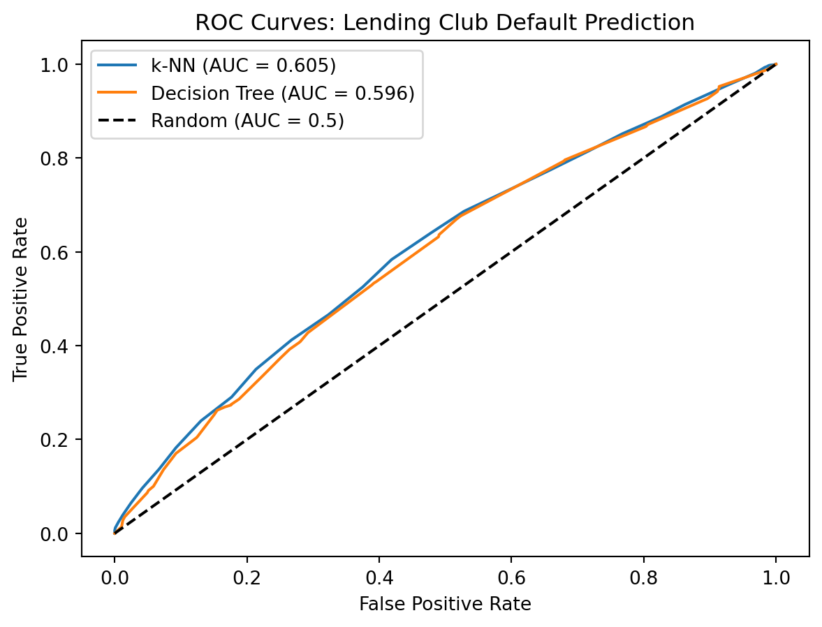
5.3 Interpreting the Tree
One of the biggest advantages of decision trees is interpretability. We can visualize the learned tree and see exactly which rules the model uses to make decisions. This is something we cannot do with k-NN — there’s no simple description of why k-NN classified a particular loan as default other than “these were its nearest neighbours.” With a tree, we can trace the path from root to leaf and read off the decision logic in plain English.
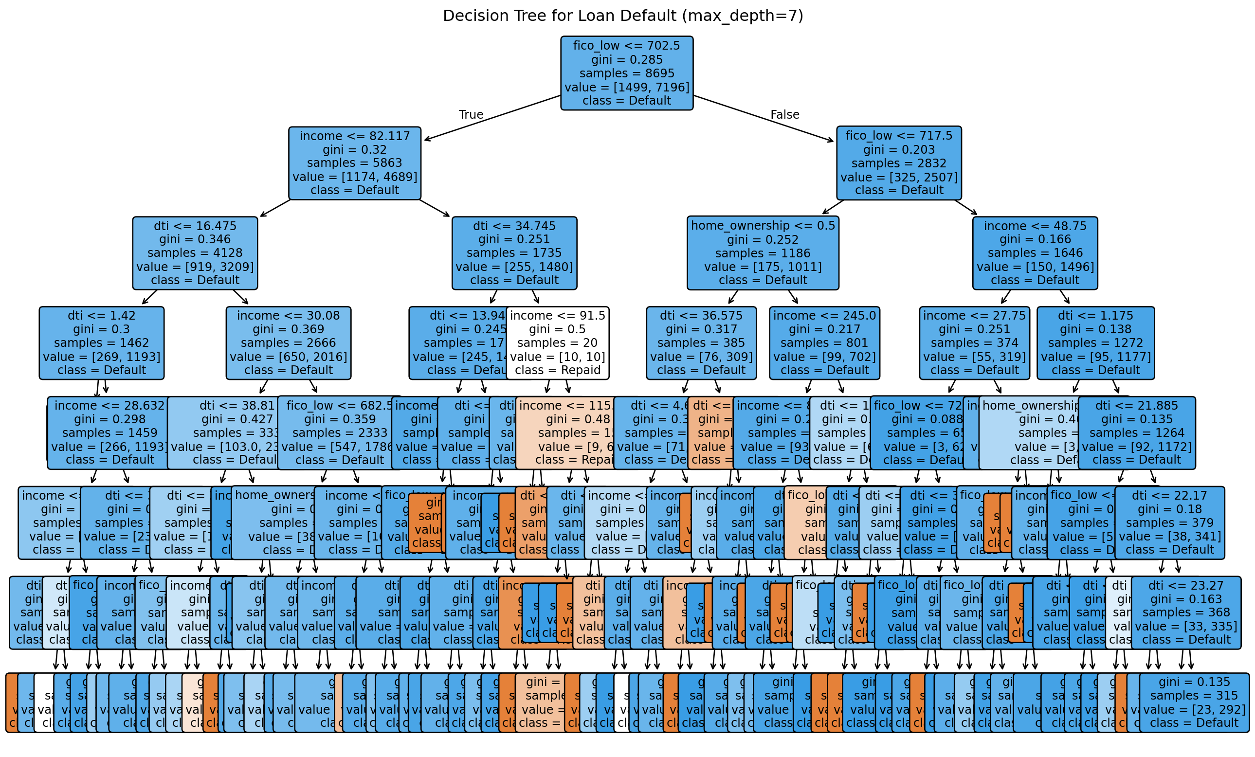
The tree reveals which features matter most. The first split (root) uses the most informative feature — the one that provides the greatest information gain when applied to the full training set. In lending data, this is typically FICO score, which is consistent with banking practice (credit score is the single most important factor in most credit decisions). Subsequent splits refine the predictions within subgroups.
We can also extract feature importances directly. Feature importance in a decision tree is computed by summing the total impurity reduction contributed by each feature across all splits in the tree. A feature that appears in many splits, especially near the top of the tree (where there are more observations to split), will have high importance. A feature that the tree never splits on has zero importance — the tree effectively decided it wasn’t useful for predicting default.
import pandas as pd

# Get feature importances from tree
importances = pd.DataFrame({
    'Feature': features,
    'Importance': tree_final.feature_importances_
}).sort_values('Importance', ascending=False)

print("Feature Importances (Decision Tree):")
print(importances.to_string(index=False))
Feature Importances (Decision Tree):
Feature Importance
dti 0.406899
income 0.294622
fico_low 0.256548
home_ownership 0.041931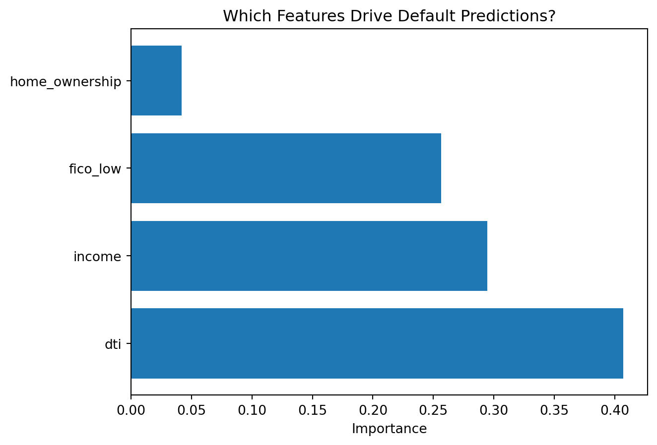
Feature importance tells us which variables the tree relied on most. Higher importance means the feature contributed more to reducing impurity across all splits in the tree. Note that feature importance is specific to the tree that was built — a different random seed or slightly different training data might produce a tree with somewhat different importances, especially for features that are similarly informative. This instability is another manifestation of the high-variance problem with individual trees.
6 Summary
This chapter introduced two nonparametric methods for classification that can learn nonlinear decision boundaries directly from data, without requiring us to specify feature transformations in advance.
k-Nearest Neighbors classifies based on majority vote among the \(k\) closest training observations. It creates flexible, curved decision boundaries that can conform to any shape. The method requires feature scaling (because distances are affected by feature magnitudes) and struggles in high dimensions due to the curse of dimensionality — as the number of features grows, the space becomes too sparse for local similarity to be meaningful. There is no training phase, but prediction is slow because every new observation must be compared to the entire training set.
Decision Trees recursively partition the data based on feature thresholds, creating axis-aligned rectangular boundaries. They are highly interpretable — you can trace the decision logic from root to leaf in plain English. They handle both numeric and categorical features without preprocessing, and they require no feature scaling. The main weakness is high variance: small changes in the training data can produce very different trees. Trees are also prone to overfitting without regularization, which is controlled by hyperparameters like maximum depth, minimum samples per leaf, or cost-complexity pruning.
Both methods use the same general strategy for selecting hyperparameters: cross-validation. For k-NN, we cross-validate over \(k\); for trees, we cross-validate over depth or pruning parameters. The bias-variance tradeoff appears in both: small \(k\) or deep trees mean high variance and low bias (risk of overfitting), while large \(k\) or shallow trees mean low variance and high bias (risk of underfitting). The lesson is the same one we’ve seen throughout the course — model complexity must be calibrated to the data.
The high variance of individual trees is a significant limitation, but it leads directly to one of the most successful ideas in machine learning: combining many trees into an ensemble. Next week, we’ll see how Random Forests and Gradient Boosting use hundreds or thousands of trees to achieve much better predictions than any single tree could.
7 References
- Cover, T., & Hart, P. (1967). Nearest neighbor pattern classification. IEEE Transactions on Information Theory, 13(1), 21-27.
- Breiman, L., Friedman, J., Stone, C. J., & Olshen, R. A. (1984). Classification and Regression Trees. CRC Press.
- Quinlan, J. R. (1986). Induction of decision trees. Machine Learning, 1(1), 81-106.
- Hastie, T., Tibshirani, R., & Friedman, J. (2009). The Elements of Statistical Learning (2nd ed.). Springer. Chapters 9, 13.