This week we move from predicting continuous outcomes (regression) to predicting categorical outcomes. This is the classification problem: given features \(\mathbf{x}\), predict which class an observation belongs to.
Classification is everywhere in finance. A bank reviewing a loan application wants to predict whether the applicant will default. A credit card company monitors transactions to flag potential fraud. An equity analyst might classify stocks into “buy,” “hold,” or “sell” categories. A risk manager needs to identify which corporate bonds are likely to be downgraded. Insurance companies classify applicants into risk tiers to set premiums. In each case, the goal is the same: use observable characteristics to predict a categorical outcome.
The simplest version is binary classification, where there are only two possible outcomes. We encode these as \(y \in \{0, 1\}\)—for example, \(y = 1\) for “default” and \(y = 0\) for “no default.” Given \(n\) observations, each with features \(\mathbf{x}_i\) and a binary class label \(y_i\), we want to learn a function that predicts \(y\) for new observations.
There are two fundamentally different ways to approach classification. The first is to predict the class directly—output 0 or 1 with no uncertainty attached. The second is to predict the probability of each class, \(P(y = 1 \,|\, \mathbf{x})\), and then threshold that probability to make a decision. The second approach is far more useful in practice because it tells us how confident we are in the prediction, not just the prediction itself.
Why does confidence matter? Consider two loan applicants, both classified as “likely to default.” If one has a 51% predicted default probability and the other has a 95% probability, a bank would treat them very differently. The first might receive the loan with extra monitoring; the second would be rejected outright. A model that outputs only “default” or “no default” loses this crucial information.
This chapter covers the two most common linear classification methods: logistic regression and linear discriminant analysis (LDA). Both produce linear decision boundaries, but they approach the problem from different angles. We’ll also study decision boundaries—the geometric interpretation of classification—and the evaluation metrics used to assess how well a classifier performs, which turn out to be surprisingly subtle when classes are imbalanced.
2 Why Not Just Use Regression?
2.1 The Linear Probability Model
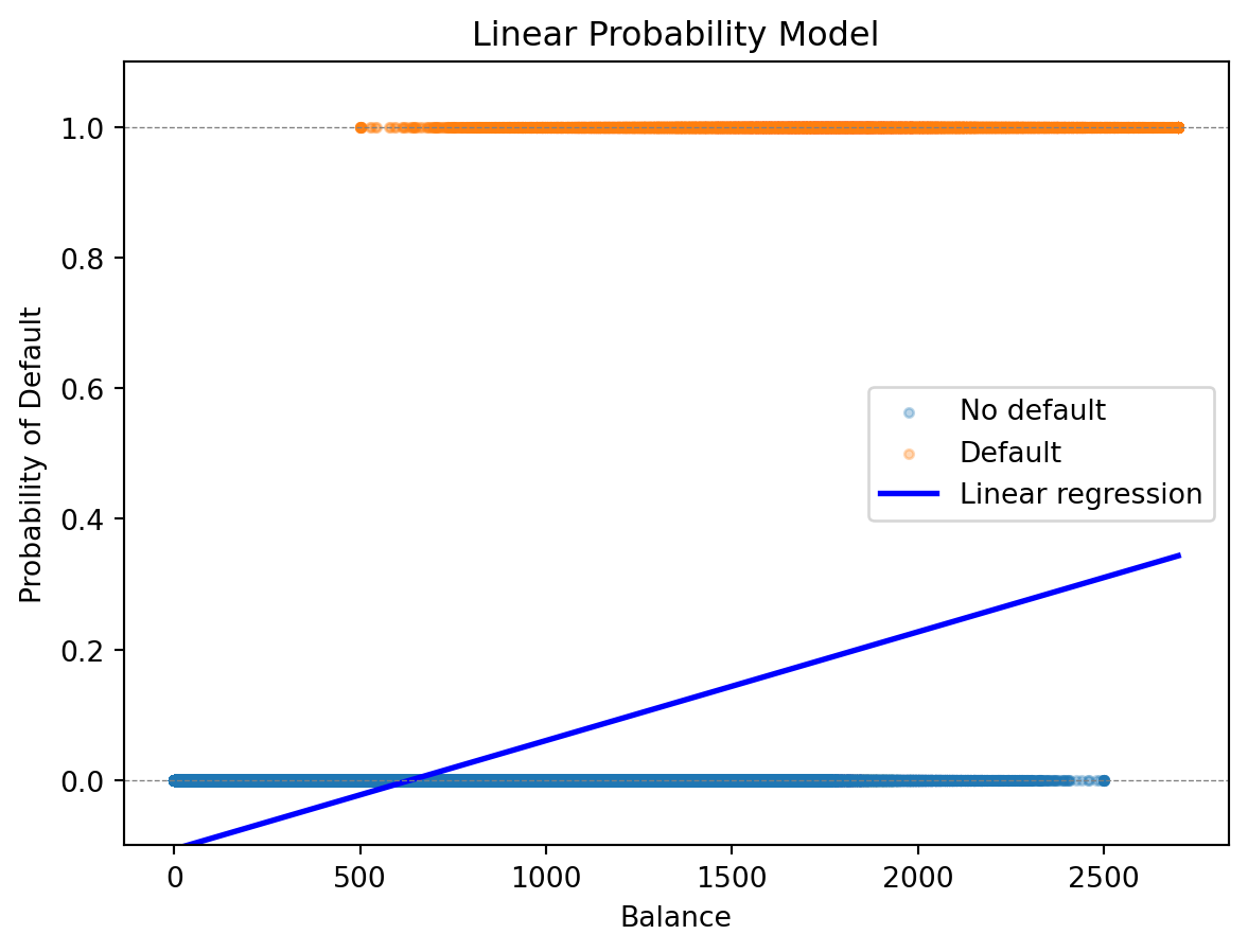
If classification is about predicting a 0/1 outcome, why not just use the regression tools we already know? This is a natural first idea: encode the class labels as numbers—\(y = 0\) for one class, \(y = 1\) for the other—and fit ordinary linear regression. The predicted values \(\hat{y}\) can then be interpreted as the probability that \(y = 1\).
This approach is called the linear probability model, and it has a long history in economics and the social sciences. It’s simple, interpretable, and uses familiar tools. But it has a fundamental flaw that becomes apparent as soon as we try it.
To illustrate, we’ll use credit card default data throughout this chapter. The dataset contains information on 1 million credit card holders: their current balance, their annual income, and whether they defaulted on their payments (1) or not (0). Our goal is to predict default from balance and income.
from sklearn.linear_model import LinearRegression# Fit linear regressionX = balance.reshape(-1, 1)y = defaultlr = LinearRegression()lr.fit(X, y)# Predictionsbalance_grid = np.linspace(0, 2700, 100).reshape(-1, 1)prob_linear = lr.predict(balance_grid)
2.2 The Problem with Linear Regression for Classification
The linear probability model has a fundamental flaw: it can produce “probabilities” that aren’t valid probabilities. By definition, probabilities must lie between 0 and 1. But linear regression is just a line (or hyperplane), and a line extends infinitely in both directions. For sufficiently extreme values of the features, the predicted “probability” will inevitably fall outside the valid range.
Minimum predicted probability: -0.106
Maximum predicted probability: 0.344
Number of predictions < 0: 330069
Number of predictions > 1: 0
What does a probability of -0.05 mean? Or 1.15? These predictions are nonsensical. A probability cannot be negative (that would mean “less likely than impossible”), nor can it exceed 1 (that would mean “more likely than certain”). Yet linear regression happily produces such values because it has no concept of the output being bounded.
This isn’t just a theoretical concern. In our credit default example, people with very low balances get negative predicted probabilities, while those with very high balances might get probabilities above 1. If we’re using these predictions to make decisions—approving or denying credit—we need values we can actually interpret.
We need a function that naturally maps any input to the interval (0, 1), no matter how extreme the features become. This function should be monotonic (higher input means higher or equal output), smooth, and easy to work with mathematically. The logistic function satisfies all these requirements, and logistic regression is built around it.
3 Logistic Regression
3.1 The Logistic Function
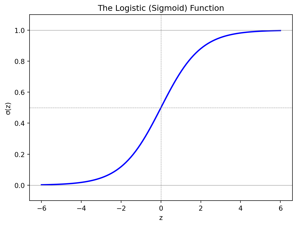
Instead of modeling probability as a linear function, logistic regression uses the logistic function (also called the sigmoid function):
The two expressions are equivalent—you can verify this by multiplying the first form by \(e^{-z}/e^{-z}\). The second form is often more convenient computationally.
This S-shaped function has exactly the properties we need for modeling probabilities. First, the output is always between 0 and 1, no matter what value we plug in for \(z\). As \(z \to -\infty\), the denominator \(1 + e^{-z}\) becomes huge (because \(e^{-z} \to \infty\)), so \(\sigma(z) \to 0\). As \(z \to +\infty\), we have \(e^{-z} \to 0\), so the denominator approaches 1 and \(\sigma(z) \to 1\). The function smoothly interpolates between these extremes.
Second, the function is monotonically increasing: larger values of \(z\) always give larger probabilities. This is intuitive—if the “evidence” for class 1 (as captured by \(z\)) increases, the probability of class 1 should increase.
Third, the function is symmetric around \(z = 0\). When \(z = 0\), we have \(\sigma(0) = 1/(1 + 1) = 0.5\)—a coin flip, maximum uncertainty. The function rises from near 0 to near 1, with the steepest part centered at this midpoint.
Fourth, the function has a nice mathematical property: its derivative has a simple form. Specifically, \(\frac{d\sigma}{dz} = \sigma(z)(1 - \sigma(z))\). This makes optimization (finding the best coefficients) more tractable.
3.2 The Logistic Regression Model
In logistic regression, we model the probability of the positive class as:
Let’s unpack this notation carefully. The expression \(P(y = 1 \,|\, \mathbf{x})\) reads “the probability that \(y = 1\) given \(\mathbf{x}\).” This is a conditional probability—the probability of default, given that we observe a particular set of feature values. The vertical bar “|” means “given” or “conditional on.” For a credit card holder with balance $2,000, we’re asking: what is the probability this specific person defaults, given their balance?
Here \(\mathbf{x} = (x_1, x_2, \ldots, x_p)'\) is a \(p\)-vector of features (attributes) for an observation. In our credit example, this might be balance and income, so \(p = 2\). The vector \(\boldsymbol{\beta} = (\beta_1, \beta_2, \ldots, \beta_p)'\) contains the corresponding coefficients we need to learn from data. The scalar \(\beta_0\) is the intercept (also called the bias term).
It helps to define \(z = \beta_0 + \boldsymbol{\beta}' \mathbf{x}\) as the linear predictor. Writing out the dot product explicitly:
This should look familiar—it’s exactly the same linear combination we used in linear regression. The difference is what we do with it. In linear regression, \(z\) is directly the predicted output. In logistic regression, \(z\) is the input to the logistic function, which then produces a probability.
The model becomes \(P(y = 1 \,|\, \mathbf{x}) = 1/(1 + e^{-z})\). Think of \(z\) as a “score” that can range from \(-\infty\) to \(+\infty\). The logistic function compresses this infinite range into the interval (0, 1):
When \(z = 0\): \(P(y=1) = 0.5\). This is the point of maximum uncertainty—a coin flip.
When \(z > 0\): \(P(y=1) > 0.5\). Positive scores indicate the observation is more likely to be class 1.
When \(z < 0\): \(P(y=1) < 0.5\). Negative scores indicate the observation is more likely to be class 0.
When \(z\) is large and positive: \(P(y=1)\) approaches 1. We’re very confident it’s class 1.
When \(z\) is large and negative: \(P(y=1)\) approaches 0. We’re very confident it’s class 0.
The coefficients \(\beta_0, \beta_1, \ldots, \beta_p\) determine how the features translate into the score \(z\). If \(\beta_1 > 0\), then higher values of \(x_1\) increase the score, which increases the probability of class 1. If \(\beta_1 < 0\), higher \(x_1\) decreases the probability. The magnitude of \(\beta_1\) determines how strongly \(x_1\) affects the probability.
3.3 Odds and Log-Odds
To interpret logistic regression coefficients, we need to understand odds. You’ve encountered odds in sports betting: “the Leafs are 3-to-1 to win” means that for every 3 times they win, they lose once. Put another way, they win 3 out of every 4 games, or 75% of the time.
Formally, odds are the ratio of the probability of an event to the probability of non-event:
Odds and probability contain the same information but express it differently. If you know one, you can compute the other. The table below shows some correspondences:
Probability
Odds
Interpretation
50%
1:1
Even money—equally likely
75%
3:1
3 times more likely to happen than not
20%
1:4
4 times more likely not to happen
90%
9:1
Very likely
99%
99:1
Almost certain
To go from odds to probability: \(P = \text{Odds}/(1 + \text{Odds})\). To go from probability to odds: \(\text{Odds} = P/(1-P)\).
Odds range from 0 (impossible) to \(\infty\) (certain), with 1 being the neutral point (50-50). This asymmetry is awkward. An event with probability 90% has odds 9:1, while an event with probability 10% has odds 1:9 (or 0.111). The odds scale is “stretched out” above 1 and “compressed” below 1.
Taking the logarithm fixes this asymmetry. The log-odds (also called the logit) is simply \(\ln(\text{Odds})\):
Log-odds of 0 means odds = 1, which means probability = 50% (maximum uncertainty)
Positive log-odds means odds > 1, which means probability > 50% (more likely than not)
Negative log-odds means odds < 1, which means probability < 50% (less likely than not)
Log-odds can range from \(-\infty\) to \(+\infty\), symmetric around 0
Now here’s the connection to logistic regression. If we solve the logistic regression model for the log-odds, we get:
In other words, logistic regression models the log-odds as a linear function of the features. This is why it’s sometimes called a “linear model”—not because the probability is linear (it isn’t), but because the log-odds is.
This gives us a clean interpretation of the coefficients. The coefficient \(\beta_j\) tells us how a one-unit increase in \(x_j\) changes the log-odds, holding other features constant:
If \(\beta_j > 0\): higher \(x_j\) increases the log-odds, which increases the probability of \(y = 1\)
If \(\beta_j < 0\): higher \(x_j\) decreases the log-odds, which decreases the probability of \(y = 1\)
If \(\beta_j = 0\): \(x_j\) has no effect on the probability
We can also interpret coefficients as odds ratios by exponentiating. If we increase \(x_j\) by one unit, the log-odds changes by \(\beta_j\), which means the odds get multiplied by \(e^{\beta_j}\). For example:
If \(\beta_j = 0.5\), then \(e^{0.5} \approx 1.65\): each one-unit increase in \(x_j\) multiplies the odds by 1.65 (a 65% increase in odds)
If \(\beta_j = -0.3\), then \(e^{-0.3} \approx 0.74\): each one-unit increase in \(x_j\) multiplies the odds by 0.74 (a 26% decrease in odds)
If \(\beta_j = 0\), then \(e^0 = 1\): the odds are unchanged
This odds ratio interpretation is common in medical research and epidemiology. You might read that “each additional year of smoking increases the odds of lung cancer by 8%,” which means the coefficient on years-smoked is \(\ln(1.08) \approx 0.077\).
3.4 Fitting Logistic Regression
How do we find the best coefficients \(\beta_0, \boldsymbol{\beta}\)? As with any machine learning model, we define a loss function that measures how badly the model fits the data, then find the coefficients that minimize this loss.
For observation \(i\) with features \(\mathbf{x}_i\) and label \(y_i\), let \(\hat{p}_i = P(y_i = 1 \,|\, \mathbf{x}_i)\) be our predicted probability. What makes a good prediction? The intuition is straightforward:
If \(y_i = 1\) (the observation actually belongs to class 1), we want \(\hat{p}_i\) close to 1
If \(y_i = 0\) (the observation actually belongs to class 0), we want \(\hat{p}_i\) close to 0
In other words, a good model assigns high probability to the class that actually occurred.
Why not just use squared error, \((y_i - \hat{p}_i)^2\), like we did in regression? We could, but it turns out to have some undesirable properties for classification. The optimization landscape has flat regions that make gradient descent slow, and the loss doesn’t penalize confident wrong predictions as severely as it should.
Instead, logistic regression uses the binary cross-entropy loss (also called log loss):
This formula looks complicated, but it’s actually quite intuitive once you break it down. For each observation, only one of the two terms is “active” (the other is multiplied by zero):
When \(y_i = 1\): the loss contribution is \(-\ln(\hat{p}_i)\). If \(\hat{p}_i = 0.99\), this is \(-\ln(0.99) \approx 0.01\) (very small, good!). If \(\hat{p}_i = 0.01\), this is \(-\ln(0.01) \approx 4.6\) (large, bad!).
When \(y_i = 0\): the loss contribution is \(-\ln(1 - \hat{p}_i)\). If \(\hat{p}_i = 0.01\), this is \(-\ln(0.99) \approx 0.01\) (very small, good!). If \(\hat{p}_i = 0.99\), this is \(-\ln(0.01) \approx 4.6\) (large, bad!).
The logarithm has a crucial property: as the predicted probability for the correct class approaches 0, the loss goes to infinity. This severely penalizes confident wrong predictions. If the model says “I’m 99% sure this is class 0” but it’s actually class 1, the loss is enormous. This encourages the model to be well-calibrated—to only be confident when it should be.
Both linear and logistic regression fit into the same ML framework: define a loss function, then minimize it. The table below compares them:
The key difference in the last row: linear regression has a closed-form solution (we can write down a formula for the optimal coefficients), but logistic regression does not. The cross-entropy loss with the logistic function creates a nonlinear optimization problem. We solve it using iterative methods like gradient descent or Newton’s method, starting from an initial guess and repeatedly improving until convergence. Fortunately, the optimization problem is convex, meaning there’s a single global minimum and we’re guaranteed to find it.
NoteConnection to statistics
In statistics, minimizing cross-entropy loss is equivalent to maximum likelihood estimation. The idea is to find parameters that make the observed data most probable. If we assume each observation is an independent Bernoulli trial with probability \(\hat{p}_i\), then the likelihood of observing our data is \(\prod_i \hat{p}_i^{y_i} (1-\hat{p}_i)^{1-y_i}\). Taking the negative log gives exactly the cross-entropy loss. Minimizing MSE is equivalent to maximum likelihood under the assumption that errors are normally distributed. Both approaches—ML and statistics—arrive at the same answer through different reasoning.
3.5 Logistic Regression in Practice
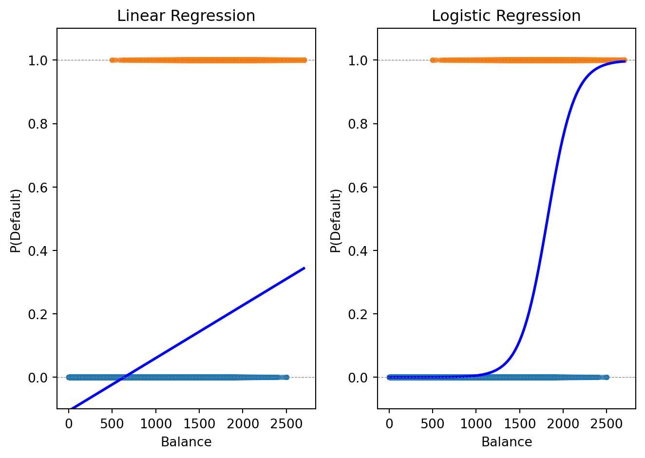
Let’s fit logistic regression to our credit default data:
from sklearn.linear_model import LogisticRegression# Fit logistic regressionlog_reg = LogisticRegression()log_reg.fit(X, y)# Predictionsprob_logistic = log_reg.predict_proba(balance_grid)[:, 1]print(f"Logistic Regression:")print(f" Intercept: {log_reg.intercept_[0]:.4f}")print(f" Coefficient on balance: {log_reg.coef_[0, 0]:.6f}")
Logistic Regression:
  Intercept: -11.6163
  Coefficient on balance: 0.006383
The logistic curve stays within [0, 1] and captures the S-shaped relationship between balance and default probability.
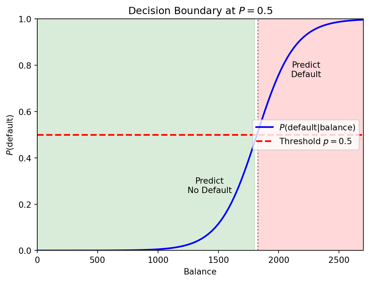
Logistic regression gives us a probability. To make a classification decision, we need a threshold (also called a cutoff). The default rule is to predict class 1 if \(P(y = 1 \,|\, \mathbf{x}) > 0.5\).
# Fit with both balance and incomeX_both = np.column_stack([balance, income])log_reg_both = LogisticRegression()log_reg_both.fit(X_both, default)print(f"Logistic Regression with Balance and Income:")print(f" Intercept: {log_reg_both.intercept_[0]:.4f}")print(f" Coefficient on balance: {log_reg_both.coef_[0, 0]:.6f}")print(f" Coefficient on income: {log_reg_both.coef_[0, 1]:.9f}")
Logistic Regression with Balance and Income:
  Intercept: -11.2532
  Coefficient on balance: 0.006383
  Coefficient on income: -0.000009279
The coefficient on income is tiny—income adds little predictive power beyond balance.
When we have \(K > 2\) classes, we can extend logistic regression using the softmax function. For each class \(k\), we define a linear predictor \(z_k = \beta_{k,0} + \boldsymbol{\beta}_k' \mathbf{x}\). The probability of class \(k\) is:
\[P(y = k | \mathbf{x}) = \frac{e^{z_k}}{\sum_{j=1}^{K} e^{z_j}}\]
This is called multinomial logistic regression or softmax regression. The softmax function ensures that each probability is between 0 and 1 and that the probabilities sum to 1 across all classes.
3.7 Regularized Logistic Regression
Just like linear regression, logistic regression can overfit—especially with many features. We can add regularization. Lasso logistic regression maximizes:
The penalty \(\lambda \sum |\beta_j|\) shrinks coefficients toward zero and can set some exactly to zero (variable selection). This prevents overfitting when \(p\) is large relative to \(n\), identifies which features matter most, and improves out-of-sample prediction. The regularization parameter \(\lambda\) is chosen by cross-validation.
from sklearn.linear_model import LogisticRegressionCV# Fit Lasso logistic regression with CVlog_reg_lasso = LogisticRegressionCV(penalty='l1', solver='saga', cv=5, max_iter=1000)log_reg_lasso.fit(X_both, default)print(f"Lasso Logistic Regression (λ chosen by CV):")print(f" Best C (inverse of λ): {log_reg_lasso.C_[0]:.4f}")print(f" Coefficient on balance: {log_reg_lasso.coef_[0, 0]:.6f}")print(f" Coefficient on income: {log_reg_lasso.coef_[0, 1]:.9f}")
Lasso Logistic Regression (λ chosen by CV):
  Best C (inverse of λ): 0.0001
  Coefficient on balance: 0.001064
  Coefficient on income: -0.000123504
4 Decision Boundaries
4.1 What Is a Decision Boundary?
Think of a classifier as drawing a line (or curve) through feature space that separates the classes. The decision boundary is this dividing line—observations on one side get predicted as Class 0, observations on the other side as Class 1.
For logistic regression with threshold 0.5, we predict Class 1 when \(P(y = 1 \,|\, \mathbf{x}) > 0.5\). The boundary is where \(P(y = 1 \,|\, \mathbf{x}) = 0.5\) exactly—the point of maximum uncertainty.
The horizontal red line marks \(P = 0.5\). Where the probability curve crosses this threshold defines the decision boundary in feature space—observations with balance above this point are predicted to default.
With multiple features, the boundary is where \(\beta_0 + \beta_1 x_1 + \beta_2 x_2 + \cdots = 0\)—a linear equation in the features. This is why logistic regression is called a linear classifier: the decision boundary is a line (in 2D) or hyperplane (in higher dimensions).
4.2 Nonlinear Decision Boundaries
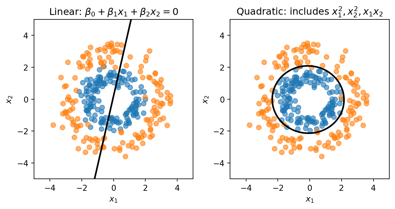
Sometimes a straight line can’t separate the classes well. We can create curved boundaries by adding transformed features to our model. If we include \(x_1^2\), \(x_2^2\), and \(x_1 x_2\) as additional features, the model is still logistic regression (linear in these new features), but the boundary is now curved in the original \((x_1, x_2)\) space.
Consider data where Class 0 forms an inner ring and Class 1 forms an outer ring. No straight line can separate these classes—we need a circular boundary. A circle centered at the origin has equation \(x_1^2 + x_2^2 = r^2\). If we add squared terms as features, the decision boundary becomes:
This is a quadratic equation in \(x_1\) and \(x_2\)—it can represent circles, ellipses, or other curved shapes.
from sklearn.preprocessing import PolynomialFeatures# Linear: uses only x1, x2log_reg_linear = LogisticRegression()log_reg_linear.fit(X_ring, y_ring)# Quadratic: add x1^2, x2^2, x1*x2 as new featurespoly = PolynomialFeatures(degree=2)X_ring_poly = poly.fit_transform(X_ring)log_reg_quad = LogisticRegression()log_reg_quad.fit(X_ring_poly, y_ring)
LogisticRegression()
In a Jupyter environment, please rerun this cell to show the HTML representation or trust the notebook. On GitHub, the HTML representation is unable to render, please try loading this page with nbviewer.org.
The linear model is forced to draw a straight line through the rings. The quadratic model can learn a circular boundary that actually separates the classes.
5 Linear Discriminant Analysis
5.1 Why Another Classifier?
Before diving into the mechanics, it helps to see where LDA fits relative to what we’ve already covered. The table below compares three approaches:
Clustering (Week 5)
Logistic Regression
LDA
Type
Unsupervised
Supervised
Supervised
Labels
Unknown — discover them
Known — learn a boundary
Known — learn distributions
Strategy
Assume each group is a distribution; find the groups
Directly model \(P(y \mid \mathbf{x})\)
Model \(P(\mathbf{x} \mid y)\) per class, then apply Bayes’ theorem
LDA is the supervised version of the distributional thinking used in clustering. In clustering, we assumed each group came from a distribution and tried to discover the groups. In LDA, we already know the groups and want to learn what makes each group different so we can classify new observations. In practice, LDA and logistic regression often give similar answers — the value is in understanding both ways of thinking about classification.
5.2 A Bayesian Approach to Classification
Logistic regression directly models \(P(y | \mathbf{x})\)—the probability of the class given the features. This is called the discriminative approach: we learn to discriminate between classes without modeling where the data comes from.
Discriminant analysis takes a fundamentally different approach. Instead of directly modeling the probability of class given features, it asks: “If I knew an observation came from class \(k\), what would its features look like?” This is called the generative approach because we’re modeling how the data is generated within each class.
Why would we do this? The key insight is Bayes’ theorem, which lets us flip conditional probabilities:
\[P(y = k | \mathbf{x}) = \frac{P(\mathbf{x} | y = k) \cdot P(y = k)}{P(\mathbf{x})}\]
Posterior\(P(y = k | \mathbf{x})\): What we want—the probability of class \(k\) given the observed features. This is what we’ll use to classify new observations.
Likelihood\(P(\mathbf{x} | y = k)\): The probability density of the features, given that the observation comes from class \(k\). This answers “what do class-\(k\) observations look like?”
Prior\(P(y = k)\): How common is class \(k\) in the population, before we observe any features? If 3% of loans default, the prior probability of default is 0.03.
Evidence\(P(\mathbf{x})\): The overall probability density of the features, regardless of class. This is a normalizing constant that ensures the posteriors sum to 1.
The generative approach has a nice interpretation. Imagine you’re trying to identify whether an email is spam or legitimate. The discriminative approach (logistic regression) asks: “Given these words, how likely is spam?” The generative approach asks: “What words do spam emails typically contain? What words do legitimate emails contain? Given my observation, which pattern is it more consistent with?”
Let’s establish notation. We have \(K\) classes labeled \(1, 2, \ldots, K\). Let \(\pi_k = P(y = k)\) be the prior probability of class \(k\), and let \(f_k(\mathbf{x}) = P(\mathbf{x} | y = k)\) be the probability density of \(\mathbf{x}\) given class \(k\). Bayes’ theorem gives us the posterior probability:
\[P(y = k | \mathbf{x}) = \frac{f_k(\mathbf{x}) \pi_k}{\sum_{j=1}^{K} f_j(\mathbf{x}) \pi_j}\]
The denominator \(\sum_{j=1}^{K} f_j(\mathbf{x}) \pi_j\) is the total probability of observing \(\mathbf{x}\) across all classes. It’s the same for all classes \(k\), so it’s just a normalizing constant that ensures the posteriors sum to 1. For classification purposes, we can often ignore it and just compare the numerators.
We classify to the class with the highest posterior probability: \(\hat{y} = \arg\max_k P(y = k | \mathbf{x})\). Since the denominator is constant across classes, this is equivalent to \(\hat{y} = \arg\max_k f_k(\mathbf{x}) \pi_k\).
5.3 The Normality Assumption
The Bayesian framework tells us how to combine the likelihood and prior, but it doesn’t tell us what the likelihood looks like. We need to specify a model for \(f_k(\mathbf{x})\)—the distribution of features within each class.
Linear Discriminant Analysis (LDA) makes a specific assumption: within each class, the features follow a multivariate normal distribution. In notation:
\[\mathbf{X} \,|\, y = k \;\sim\; \mathcal{N}(\boldsymbol{\mu}_k, \boldsymbol{\Sigma})\]
This says: “If an observation belongs to class \(k\), its features are drawn from a multivariate normal distribution with mean \(\boldsymbol{\mu}_k\) and covariance matrix \(\boldsymbol{\Sigma}\).”
\(\boldsymbol{\mu}_k\) is the mean vector of class \(k\). Different classes have different centers.
\(\boldsymbol{\Sigma}\) is the covariance matrix. It describes the shape (how spread out, how correlated) of each class.
The term \((\mathbf{x} - \boldsymbol{\mu}_k)' \boldsymbol{\Sigma}^{-1}(\mathbf{x} - \boldsymbol{\mu}_k)\) is the squared Mahalanobis distance from \(\mathbf{x}\) to the class center \(\boldsymbol{\mu}_k\). Points far from the center have lower density.
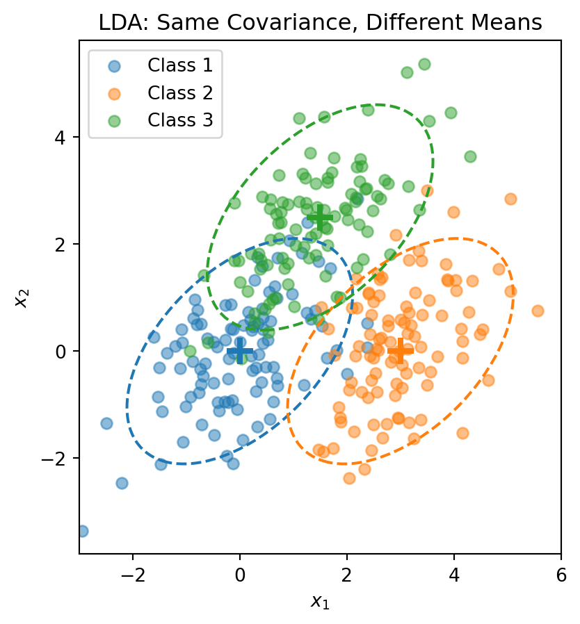
The critical assumption in LDA is that all classes share the same covariance matrix \(\boldsymbol{\Sigma}\). This means each class is a normal “blob” with its own center \(\boldsymbol{\mu}_k\), but all the blobs have the same shape—the same orientation, the same spread in each direction, the same correlations between features. Only the centers differ.
Why make this assumption? It dramatically reduces the number of parameters we need to estimate. A covariance matrix for \(p\) features has \(p(p+1)/2\) unique entries. With \(K\) classes, allowing separate covariances would require estimating \(K \times p(p+1)/2\) parameters. With shared covariance, we only estimate \(p(p+1)/2\) parameters (plus the \(K\) mean vectors). When \(p\) is large or \(n\) is small, this parsimony matters a lot.
The dashed ellipses show the 95% probability contours—they have the same shape (orientation and spread) but different centers.
5.4 The Discriminant Function
Start with the posterior from Bayes’ theorem:
\[P(y = k \,|\, \mathbf{x}) = \frac{f_k(\mathbf{x}) \pi_k}{\sum_{j=1}^{K} f_j(\mathbf{x}) \pi_j}\]
Taking the log and plugging in the normal density:
\[\ln P(y = k \,|\, \mathbf{x}) = \ln f_k(\mathbf{x}) + \ln \pi_k - \underbrace{\ln \sum_{j} f_j(\mathbf{x}) \pi_j}_{\text{same for all } k}\]
The normal density gives \(\ln f_k(\mathbf{x}) = -\frac{p}{2}\ln(2\pi) - \frac{1}{2}\ln|\boldsymbol{\Sigma}| - \frac{1}{2}(\mathbf{x} - \boldsymbol{\mu}_k)'\boldsymbol{\Sigma}^{-1}(\mathbf{x} - \boldsymbol{\mu}_k)\).
The first two terms don’t depend on \(k\) (shared covariance!). Expanding the quadratic and dropping terms that don’t depend on \(k\), we get the discriminant function:
This is a scalar—one number for each class \(k\). We classify \(\mathbf{x}\) to the class with the largest discriminant: \(\hat{y} = \arg\max_k \delta_k(\mathbf{x})\).
The discriminant function is linear in \(\mathbf{x}\)—that’s why it’s called Linear Discriminant Analysis.
5.5 Decision Boundaries and Parameter Estimation
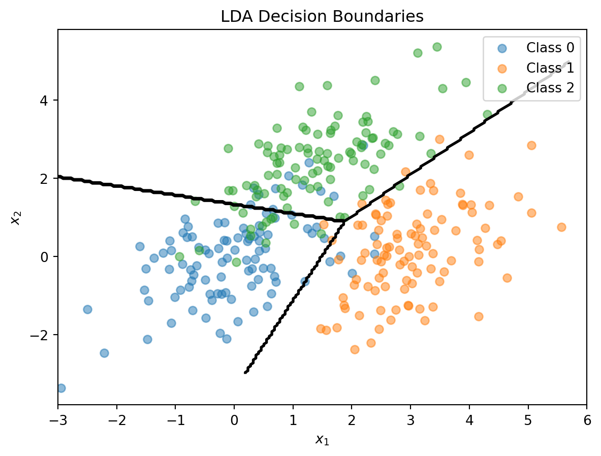
The decision boundary between classes \(k\) and \(\ell\) is where \(\delta_k(\mathbf{x}) = \delta_\ell(\mathbf{x})\). This simplifies to:
This is a linear equation in \(\mathbf{x}\)—so the boundary is a line (in 2D) or hyperplane (in higher dimensions). With \(K\) classes, we have \(K(K-1)/2\) pairwise boundaries, but only \(K-1\) of them matter for defining the decision regions.
In practice, we estimate the parameters from training data. The prior probabilities are estimated as \(\hat{\pi}_k = n_k/n\), where \(n_k\) is the number of training observations in class \(k\). The class means are estimated as \(\hat{\boldsymbol{\mu}}_k = \frac{1}{n_k} \sum_{i: y_i = k} \mathbf{x}_i\). The pooled covariance matrix is:
The pooled covariance averages within-class covariances, weighted by class size.
5.6 The LDA Recipe
It’s worth stepping back and summarizing how LDA works as a complete method:
LDA
Model
Each class \(k\) is a multivariate normal: \(\mathbf{x} \mid y = k \;\sim\; \mathcal{N}(\boldsymbol{\mu}_k,\, \boldsymbol{\Sigma})\)
Parameters
Priors \(\hat{\pi}_k = n_k / n\), means \(\hat{\boldsymbol{\mu}}_k\), pooled covariance \(\hat{\boldsymbol{\Sigma}}\)
“Loss function”
Not a loss function — parameters are estimated directly from the data (sample proportions, sample means, pooled covariance)
Classification rule
Assign \(\mathbf{x}\) to the class with the largest discriminant \(\delta_k(\mathbf{x})\)
No optimization loop, no gradient descent. LDA computes its parameters in closed form — plug in the training data and you’re done. This is fundamentally different from logistic regression, which iteratively searches for the coefficients that minimize cross-entropy loss.
5.7 LDA in Python
from sklearn.discriminant_analysis import LinearDiscriminantAnalysis# Combine the 3-class dataX_lda = np.vstack([X1, X2, X3])y_lda = np.array([0] * n_per_class + [1] * n_per_class + [2] * n_per_class)# Fit LDAlda = LinearDiscriminantAnalysis()lda.fit(X_lda, y_lda)print("LDA Class Means:")for k inrange(3):print(f" Class {k}: {lda.means_[k]}")print(f"\nClass Priors: {lda.priors_}")
LDA Class Means:
  Class 0: [ 0.00962094 -0.02608294]
  Class 1: [3.00835928 0.12294623]
  Class 2: [1.40152169 2.3715806 ]

Class Priors: [0.33333333 0.33333333 0.33333333]
5.8 Quadratic Discriminant Analysis
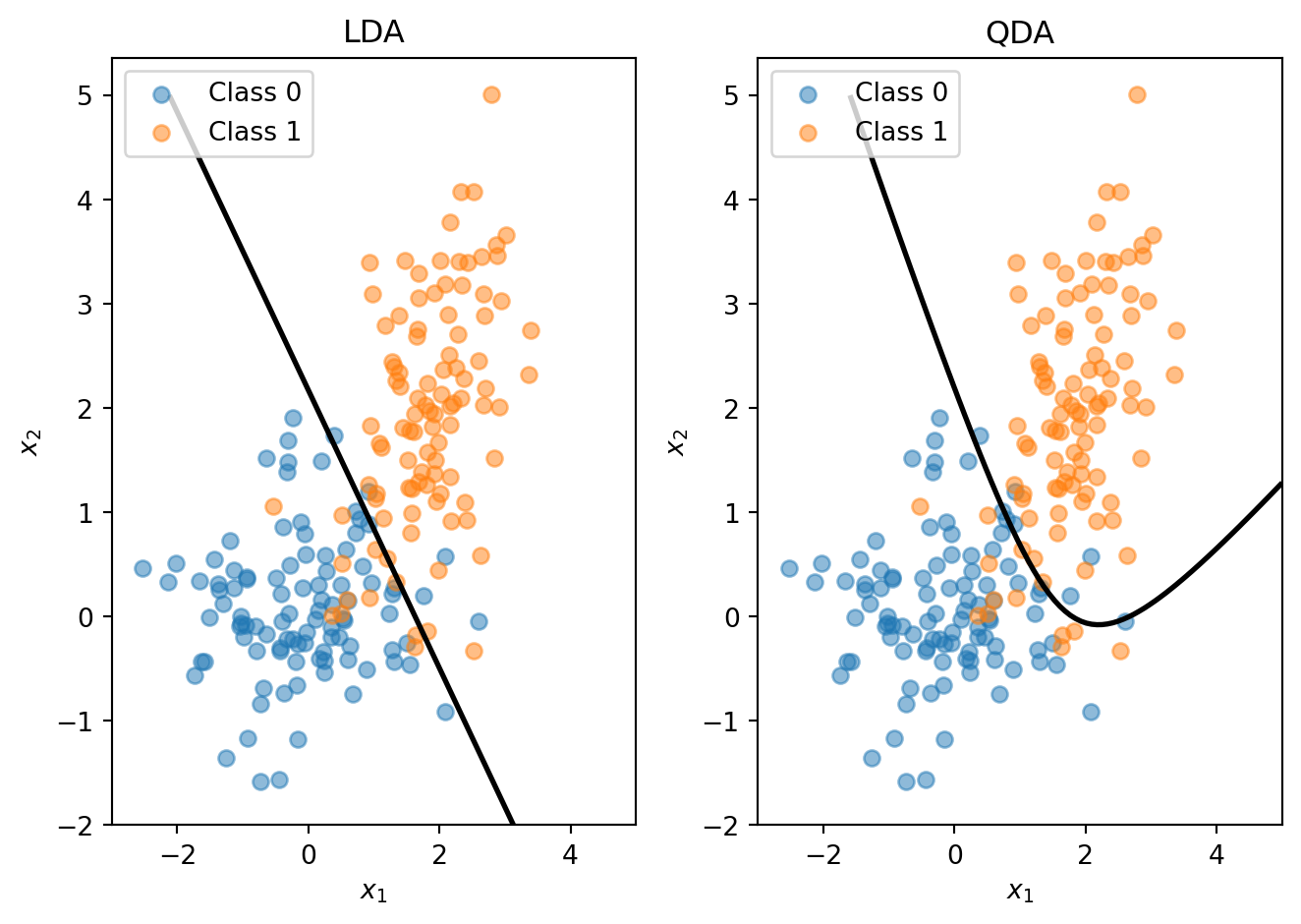
LDA assumes all classes share the same covariance matrix \(\boldsymbol{\Sigma}\). Quadratic Discriminant Analysis (QDA) relaxes this: each class has its own covariance \(\boldsymbol{\Sigma}_k\). The discriminant function becomes:
This is quadratic in \(\mathbf{x}\), giving curved decision boundaries. There is a trade-off between the methods: LDA has more restrictive assumptions, fewer parameters to estimate, and is more stable; QDA is more flexible, has more parameters, and can overfit with small samples.
When classes have different covariances, QDA captures the curved boundary while LDA is forced to use a straight line.
5.9 When to Use LDA vs. Logistic Regression
LDA and QDA have good track records as classifiers, not necessarily because the normality assumption is correct, but because estimating fewer parameters (shared \(\boldsymbol{\Sigma}\)) reduces variance, the decision boundary often works well even when normality is violated, and there is a closed-form solution with no iterative optimization needed.
When to use which: use LDA when you have limited data or classes are well-separated, use QDA when you have more data and suspect different class shapes, and consider regularized discriminant analysis to blend between LDA and QDA.
Both LDA and logistic regression produce linear decision boundaries. Logistic regression makes no assumption about the distribution of \(\mathbf{x}\), is more robust when the normality assumption is violated, and is preferred when you have binary features or mixed feature types. LDA is more efficient when normality holds (uses information about class distributions), can be more stable with small samples, and naturally handles multi-class problems. In practice, they often give similar results. Try both and compare via cross-validation.
6 Evaluating Classification Models
6.1 Beyond Accuracy
For regression, we use MSE or \(R^2\) to measure how well a model predicts continuous outcomes. Classification requires different metrics because the outcomes are categories, not numbers.
The most obvious metric is accuracy—the percentage of predictions that are correct:
where TP, TN, FP, and FN are the counts in the confusion matrix (defined below). An accuracy of 95% sounds good: we’re right 19 times out of 20!
But accuracy can be deeply misleading, especially when classes are imbalanced—meaning one class is much more common than the other. In finance, imbalanced classes are the norm, not the exception:
Credit card fraud: ~0.1% of transactions are fraudulent
Loan defaults: ~3-5% of loans default
Bankruptcy: <1% of firms go bankrupt in a given year
Extreme market moves: <5% of days have returns beyond 2 standard deviations
Consider a fraud detection model where only 0.1% of transactions are actually fraudulent. A model that predicts “not fraud” for every single transaction achieves 99.9% accuracy! It’s correct on all the legitimate transactions (99.9% of the data) and wrong only on the frauds (0.1% of the data). This “model” is useless—it catches zero frauds, which was the entire point.
The problem is that accuracy treats all errors equally. In fraud detection, a false negative (missing a fraud) costs far more than a false positive (investigating a legitimate transaction). In medical diagnosis, missing a cancer might be fatal, while a false alarm leads to more tests. We need metrics that distinguish between types of errors.
6.2 The Confusion Matrix
The confusion matrix organizes all the ways a classifier can be right or wrong. For binary classification, there are exactly four possibilities:
Actual Positive
Actual Negative
Predicted Positive
True Positive (TP)
False Positive (FP)
Predicted Negative
False Negative (FN)
True Negative (TN)
Let’s define each cell:
True Positive (TP): We predicted positive, and it actually was positive. In fraud detection: we flagged a transaction as fraud, and it really was fraud. This is a correct positive prediction.
False Positive (FP): We predicted positive, but it was actually negative. In fraud detection: we flagged a transaction as fraud, but it was legitimate. This is a false alarm, also called a Type I error. The “positive” part refers to what we predicted, not whether it’s good.
True Negative (TN): We predicted negative, and it actually was negative. In fraud detection: we said “not fraud,” and it was indeed not fraud. This is a correct negative prediction.
False Negative (FN): We predicted negative, but it was actually positive. In fraud detection: we said “not fraud,” but it actually was fraud. We missed a real positive. This is also called a Type II error.
Memory tip: The first word (True/False) tells you if the prediction was correct. The second word (Positive/Negative) tells you what you predicted.
Different applications care about different cells. In credit card fraud detection, false negatives are very costly (the bank loses money on undetected fraud), while false positives are just annoying (a legitimate customer gets a call). In airport security screening, false negatives are catastrophic (a threat gets through), so we tolerate many false positives (innocent passengers get extra screening).
From the confusion matrix, we can compute several metrics that capture different aspects of performance:
Accuracy is the overall correct rate: \[\text{Accuracy} = \frac{TP + TN}{TP + TN + FP + FN}\] This is the fraction of all predictions that were correct. As discussed, it can be misleading with imbalanced classes.
Precision answers: “Of those we predicted positive, how many actually are?” \[\text{Precision} = \frac{TP}{TP + FP}\] High precision means few false alarms. If our fraud detector has 90% precision, then 9 out of 10 transactions we flag are actually fraudulent.
Recall (also called sensitivity or true positive rate) answers: “Of the actual positives, how many did we catch?” \[\text{Recall} = \frac{TP}{TP + FN}\] High recall means we catch most of the positives. If our fraud detector has 80% recall, we catch 80% of actual frauds.
Specificity (also called true negative rate) answers: “Of the actual negatives, how many did we correctly identify?” \[\text{Specificity} = \frac{TN}{TN + FP}\] High specificity means few legitimate observations are flagged as positive.
False Positive Rate is the complement of specificity: \[\text{FPR} = \frac{FP}{TN + FP} = 1 - \text{Specificity}\] This is the fraction of negatives that we incorrectly labeled as positive.
from sklearn.metrics import confusion_matrix, classification_report# Using our credit default data with logistic regressiony_pred = log_reg.predict(X)# Confusion matrixcm = confusion_matrix(default, y_pred)print("Confusion Matrix:")print(f" Predicted No Predicted Yes")print(f" Actual No {cm[0,0]:5d}{cm[0,1]:5d}")print(f" Actual Yes {cm[1,0]:5d}{cm[1,1]:5d}")
Confusion Matrix:
                  Predicted No  Predicted Yes
  Actual No          961793          5207
  Actual Yes         19202         13798
In our credit default example, about 97% of cardholders don’t default and only 3% do. Using the standard threshold of 0.5, the model rarely predicts “default” because the probability of default is below 0.5 for most people. We get high accuracy (97%+) but low recall—we miss most actual defaults.
Is this a good model? It depends on what you care about. For a credit card company, missing a default is costly—the company loses the unpaid balance. A false alarm (flagging someone who won’t default) is much cheaper—maybe the company offers them a lower credit limit or higher interest rate. Given this asymmetry, the company would rather catch more actual defaults (higher recall) even if it means more false alarms (lower precision).
The key insight is that the 0.5 threshold isn’t sacred. Logistic regression gives us a probability, and we choose how to convert that probability into a decision. Instead of predicting “default” when \(P(\text{default}) > 0.5\), we can use any threshold \(\tau\):
\[\text{Predict default if } P(\text{default}) > \tau\]
Lowering the threshold has predictable effects:
More observations cross the threshold, so we predict “positive” (default) more often
We catch more actual positives → higher recall
We also flag more negatives by mistake → more false positives, lower precision
Overall accuracy may drop because we’re wrong on many negatives
Raising the threshold has the opposite effects:
Fewer observations cross the threshold, so we predict “positive” less often
We catch fewer actual positives → lower recall
We have fewer false positives → higher precision
There’s a fundamental trade-off between precision and recall. A very low threshold (like 0.01) gives nearly perfect recall—we catch almost all defaults—but terrible precision because we flag almost everyone. A very high threshold (like 0.99) gives nearly perfect precision—when we flag someone, they almost certainly will default—but terrible recall because we catch almost nobody.
The “right” threshold depends on the relative costs of false positives and false negatives, which varies by application.
Lowering the threshold from 0.5 to 0.1 dramatically increases recall (catching defaults) at the cost of more false positives.
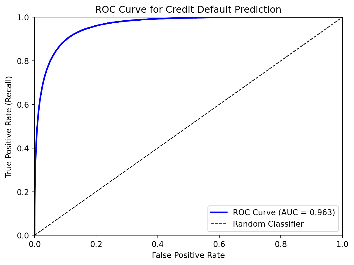
6.4 The ROC Curve
How do we visualize the precision-recall (or equivalently, TPR-FPR) trade-off across all possible thresholds? The Receiver Operating Characteristic (ROC) curve does exactly this.
Each point on the curve corresponds to a different threshold. As we vary the threshold from 1 (predict nothing positive) to 0 (predict everything positive), we trace out the curve.
At threshold = 1, we predict everything negative: TPR = 0 (catch no positives) and FPR = 0 (no false positives). This is the bottom-left corner.
At threshold = 0, we predict everything positive: TPR = 1 (catch all positives) and FPR = 1 (all negatives are false positives). This is the top-right corner.
As we lower the threshold, we move along the curve from bottom-left toward top-right. The shape of this curve tells us about classifier quality:
Good classifiers hug the top-left corner. They achieve high TPR (catch most positives) with low FPR (few false positives). The curve rises steeply at first.
Random classifiers follow the diagonal line from (0,0) to (1,1). A random guess has no discriminative power—increasing TPR requires proportionally increasing FPR.
Perfect classifiers go straight up to (0,1) and then across to (1,1). They can catch all positives (TPR=1) with zero false positives (FPR=0).
The ROC curve separates model quality from threshold choice. Two models might have the same accuracy at threshold 0.5, but very different ROC curves. The one with the better curve has more flexibility—it can achieve higher recall without sacrificing as much precision.
The Area Under the Curve (AUC) summarizes the entire ROC curve in a single number. It’s literally the area under the ROC curve:
AUC = 1.0: Perfect classifier. The ROC curve goes straight up and then across, enclosing the entire unit square.
AUC = 0.5: Random guessing. The ROC curve follows the diagonal, enclosing exactly half the square.
AUC < 0.5: Worse than random. This usually means the predictions are inverted—swap 0 and 1 and you’d do better.
There’s a beautiful probabilistic interpretation: AUC equals the probability that a randomly chosen positive example has a higher predicted probability than a randomly chosen negative example. In other words, if we picked one defaulter and one non-defaulter at random, what’s the chance our model ranks the defaulter higher?
This interpretation makes AUC intuitive. An AUC of 0.85 means: pick a random defaulter and a random non-defaulter; 85% of the time, the model assigns higher default probability to the defaulter. The model usually ranks correctly.
from sklearn.metrics import roc_auc_scoreauc = roc_auc_score(default, prob_pred)print(f"AUC for credit default model: {auc:.3f}")
AUC for credit default model: 0.963
AUC is useful for comparing models because it’s threshold-independent. Two models with the same AUC have equally good ranking ability, even if their optimal thresholds differ. It answers: “How well does the model separate positives from negatives?” rather than “How accurate is the model at a specific threshold?”
However, AUC has limitations. It treats all false positive rates equally, but in practice you might only care about the low-FPR region (because you can’t tolerate many false alarms). A model that’s great at low FPR but poor at high FPR might have the same AUC as a model with the opposite pattern. For this reason, some practitioners prefer partial AUC (area under a specific region) or precision-recall curves.
6.5 Choosing the Optimal Threshold
The “best” threshold depends on the costs of different errors. Let \(c_{FN}\) be the cost of a false negative (missing a default) and \(c_{FP}\) be the cost of a false positive (false alarm). If missing defaults is very costly (e.g., the bank loses the loan amount), we want a lower threshold to maximize recall.
The objective is to minimize total cost: \[\text{Total Cost} = c_{FN} \cdot FN + c_{FP} \cdot FP\]
Or equivalently, maximize: \[\text{Benefit} = TP - c \cdot FP\]
where \(c = c_{FP} / c_{FN}\) is the relative cost ratio.
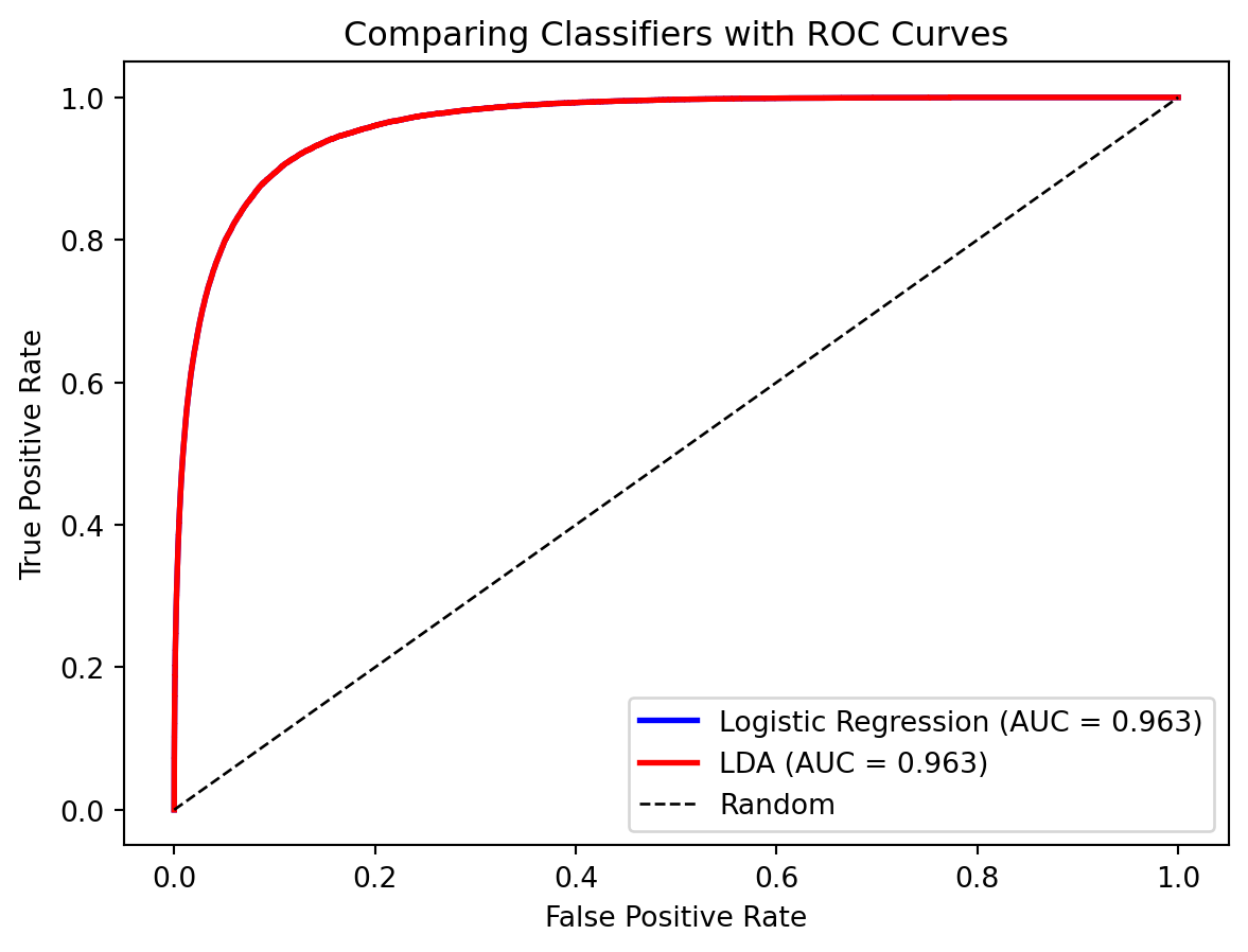
6.6 Comparing Classifiers
The ROC curves are nearly identical—both methods perform similarly on this dataset. The AUC provides a single number for comparison.
7 Summary
Classification predicts categorical outcomes and is a core supervised learning task. The linear probability model (regression with 0/1 outcome) fails because it can produce impossible probabilities.
Logistic regression uses the sigmoid function to model probabilities properly. Outputs are always in (0, 1), coefficients measure effect on log-odds, and the model can be regularized (Lasso) for variable selection.
Linear Discriminant Analysis takes a Bayesian approach. It models class-conditional distributions as normal and assumes shared covariance (LDA) or class-specific covariance (QDA). LDA often performs similarly to logistic regression in practice.
Accuracy can be misleading with imbalanced classes. The confusion matrix breaks down predictions into TP, FP, TN, FN. Precision (of predicted positives, how many are correct?) and Recall (of actual positives, how many did we catch?) capture different aspects of performance. The ROC curve shows the trade-off across all thresholds, and AUC summarizes discriminative ability in a single number. The optimal threshold depends on the costs of different types of errors.
8 References
Fisher, R. A. (1936). The use of multiple measurements in taxonomic problems. Annals of Eugenics, 7(2), 179-188.
Hastie, T., Tibshirani, R., & Friedman, J. (2009). The Elements of Statistical Learning (2nd ed.). Springer. Chapter 4.
James, G., Witten, D., Hastie, T., & Tibshirani, R. (2021). An Introduction to Statistical Learning (2nd ed.). Springer. Chapter 4.