Linear Algebra for Quantitative Finance

RSM338: Machine Learning in Finance

1 Vectors, Operations, and the Dot Product

This reference covers linear algebra from a purely computational and algebraic perspective. The question we’re answering is: what do these operations actually do to the numbers, and why would you ever want to do them?

The short answer: matrices let you batch linear operations. If you know how to do one dot product, matrix multiplication lets you do thousands of them at once. That’s the whole idea. Everything else—transpose, inverse, determinant—is machinery that supports it.

A vector is an ordered list of numbers. When we write \[\mathbf{x} = \begin{bmatrix} 3 \\ 1 \\ 4 \end{bmatrix},\] we mean \(\mathbf{x}\) is a list with three entries: the first is 3, the second is 1, the third is 4. The notation \(\mathbf{x} \in \mathbb{R}^3\) says “\(\mathbf{x}\) is a list of 3 real numbers.” More generally, \(\mathbf{x} \in \mathbb{R}^n\) means \(\mathbf{x}\) has \(n\) entries, and we use subscripts to refer to them: \(x_1\) is the first, \(x_2\) the second, and so on. In Python, a vector is a NumPy array:

import numpy as np

x = np.array([3, 1, 4])
print(f"x = {x}, has {len(x)} entries")
print(f"First entry x[0] = {x[0]}")  # Python indexes from 0

x = [3 1 4], has 3 entries
First entry x[0] = 3

You can add two vectors of the same length entry-by-entry. If \[\mathbf{x} = \begin{bmatrix} 1 \\ 2 \\ 3 \end{bmatrix}, \quad \mathbf{y} = \begin{bmatrix} 4 \\ 5 \\ 6 \end{bmatrix},\] then \[\mathbf{x} + \mathbf{y} = \begin{bmatrix} 1+4 \\ 2+5 \\ 3+6 \end{bmatrix} = \begin{bmatrix} 5 \\ 7 \\ 9 \end{bmatrix}.\] You can multiply by a scalar (a single number) to scale every entry: \[3 \cdot \mathbf{x} = \begin{bmatrix} 3 \\ 6 \\ 9 \end{bmatrix}.\] Both work exactly as you’d expect in NumPy:

x = np.array([1, 2, 3])
y = np.array([4, 5, 6])

print(f"x + y = {x + y}")
print(f"3 * x = {3 * x}")

x + y = [5 7 9]
3 * x = [3 6 9]

The operation that matters most is the dot product. It takes two vectors of the same length, multiplies corresponding entries, and adds the results to produce a single number: \[\mathbf{x} \cdot \mathbf{y} = x_1 y_1 + x_2 y_2 + \cdots + x_n y_n = \sum_{i=1}^{n} x_i y_i\]

Let’s compute one by hand. Take \[\mathbf{x} = \begin{bmatrix} 2 \\ 3 \\ 1 \end{bmatrix}, \quad \mathbf{y} = \begin{bmatrix} 4 \\ 0 \\ 5 \end{bmatrix}.\] Multiply entry-by-entry: \(2 \times 4 = 8\), then \(3 \times 0 = 0\), then \(1 \times 5 = 5\). Add them up: \(8 + 0 + 5 = 13\). Two vectors go in, one number comes out. In code, the @ operator does this:

x = np.array([2, 3, 1])
y = np.array([4, 0, 5])

print(f"x @ y = {x @ y}")
print(f"Step by step: {2*4} + {3*0} + {1*5} = {2*4 + 3*0 + 1*5}")

x @ y = 13
Step by step: 8 + 0 + 5 = 13

The math and the code compute the same thing. The @ operator is just shorthand for “multiply corresponding entries and sum.” You’ll also see np.dot(x, y), which does the same thing, but @ is shorter.

You’ll often see the dot product written as \(\mathbf{x}^\top\mathbf{y}\) (read: “\(\mathbf{x}\) transpose times \(\mathbf{y}\)”). We’ll define transpose properly in the next section, but the idea is straightforward: \(\mathbf{x}\) is a column vector (size \(n \times 1\)), and \(\mathbf{x}^\top\) flips it into a row (size \(1 \times n\)). Then \(\mathbf{x}^\top\mathbf{y}\) is a matrix multiplication of a \((1 \times n)\) row times an \((n \times 1)\) column, which produces a \((1 \times 1)\) result—a single number, exactly the dot product. The dimensions have to match: the “inner” dimensions (the two \(n\)s) must be equal, and the “outer” dimensions (\(1\) and \(1\)) give you the size of the result. This dimension-matching rule will come up again and again.

The dot product shows up constantly. In regression, each observation’s predicted value \(\hat{y}_i\) is a dot product of that observation’s features with the coefficient vector. In portfolio theory, the portfolio return is a dot product of weights and returns. Once you recognize that, the natural next question is: what if I want to compute many dot products at once?

2 Matrices as Batched Dot Products

A matrix is a rectangular grid of numbers arranged in rows and columns. When we write \[\mathbf{A} = \begin{bmatrix} 1 & 2 & 3 \\ 4 & 5 & 6 \end{bmatrix},\] we mean \(\mathbf{A}\) has 2 rows and 3 columns—a “\(2 \times 3\) matrix,” written \(\mathbf{A} \in \mathbb{R}^{2 \times 3}\). The entry in row \(i\), column \(j\) is \(A_{ij}\), so \(A_{12} = 2\) and \(A_{21} = 4\). A vector is just a matrix with one column: a vector in \(\mathbb{R}^3\) is the same thing as a \(3 \times 1\) matrix.

A = np.array([[1, 2, 3],
              [4, 5, 6]])
print(f"Shape: {A.shape}")       # (2, 3) = 2 rows, 3 columns
print(f"A[0, 2] = {A[0, 2]}")   # row 1, column 3 (0-indexed)

Shape: (2, 3)
A[0, 2] = 3

But a matrix is more than a grid of numbers. Think of it as a collection of vectors stacked together: each row is a vector, and each column is a vector. This is how we use matrices in practice—when you have many vectors that you want to operate on simultaneously, you stack them into a matrix.

The transpose \(\mathbf{A}^\top\) (also written \(\mathbf{A}'\)) flips rows and columns. If \(\mathbf{A}\) is \(m \times n\), then \(\mathbf{A}^\top\) is \(n \times m\): \[\begin{bmatrix} 1 & 2 & 3 \\ 4 & 5 & 6 \end{bmatrix}^\top = \begin{bmatrix} 1 & 4 \\ 2 & 5 \\ 3 & 6 \end{bmatrix}.\] For a column vector, the transpose turns it into a row: \[\begin{bmatrix} 1 \\ 2 \\ 3 \end{bmatrix}^\top = \begin{bmatrix} 1 & 2 & 3 \end{bmatrix}.\] This is how the dot product notation \(\mathbf{x}^\top\mathbf{y}\) works: transpose \(\mathbf{x}\) from \((n \times 1)\) to \((1 \times n)\), then multiply by \(\mathbf{y}\) which is \((n \times 1)\). The inner dimensions match (\(n = n\)), and the result is \((1 \times 1)\)—a scalar.

One useful rule: the transpose of a product reverses the order: \[(\mathbf{A}\mathbf{B})^\top = \mathbf{B}^\top\mathbf{A}^\top.\] The same idea extends to longer chains: \((\mathbf{A}\mathbf{B}\mathbf{C})^\top = \mathbf{C}^\top\mathbf{B}^\top\mathbf{A}^\top\). This will come up when we derive OLS.

In code, transpose is .T:

A = np.array([[1, 2, 3], [4, 5, 6]])
print(f"A (shape {A.shape}):\n{A}")
print(f"\nA.T (shape {A.T.shape}):\n{A.T}")

A (shape (2, 3)):
[[1 2 3]
 [4 5 6]]

A.T (shape (3, 2)):
[[1 4]
 [2 5]
 [3 6]]

Now for the central idea. Suppose you have a vector \[\boldsymbol{\beta} = \begin{bmatrix} 5 \\ 3 \end{bmatrix}\] and you want to dot it with three different vectors: \[\mathbf{x}_1 = \begin{bmatrix} 3 \\ 1 \end{bmatrix}, \quad \mathbf{x}_2 = \begin{bmatrix} 0 \\ 4 \end{bmatrix}, \quad \mathbf{x}_3 = \begin{bmatrix} 2 \\ 2 \end{bmatrix}.\] You could do each one separately: \(\mathbf{x}_1^\top\boldsymbol{\beta} = 3(5) + 1(3) = 18\), then \(\mathbf{x}_2^\top\boldsymbol{\beta} = 0(5) + 4(3) = 12\), then \(\mathbf{x}_3^\top\boldsymbol{\beta} = 2(5) + 2(3) = 16\). Or you could stack the three vectors as rows of a matrix and compute all three at once:

\[\underbrace{\begin{bmatrix} 3 & 1 \\ 0 & 4 \\ 2 & 2 \end{bmatrix}}_{\mathbf{X}} \underbrace{\begin{bmatrix} 5 \\ 3 \end{bmatrix}}_{\boldsymbol{\beta}} = \begin{bmatrix} 3(5) + 1(3) \\ 0(5) + 4(3) \\ 2(5) + 2(3) \end{bmatrix} = \begin{bmatrix} 18 \\ 12 \\ 16 \end{bmatrix}\]

Each entry of the output is the dot product of one row of \(\mathbf{X}\) with \(\boldsymbol{\beta}\). Check the dimensions: \(\mathbf{X}\) is \((3 \times 2)\) and \(\boldsymbol{\beta}\) is \((2 \times 1)\). The inner dimensions match (\(2 = 2\)), and the outer dimensions give the result size: \((3 \times 1)\)—a 3-entry vector, one entry per row of \(\mathbf{X}\). That’s all matrix-vector multiplication is: the same dot product, computed against every row simultaneously. In code:

X = np.array([[3, 1],
              [0, 4],
              [2, 2]])
beta = np.array([5, 3])

# All three dot products at once
print(f"X @ beta = {X @ beta}")

# Verify: same as doing them one at a time
print(f"Row 0: {3*5 + 1*3} = {X[0] @ beta}")
print(f"Row 1: {0*5 + 4*3} = {X[1] @ beta}")
print(f"Row 2: {2*5 + 2*3} = {X[2] @ beta}")

X @ beta = [18 12 16]
Row 0: 18 = 18
Row 1: 12 = 12
Row 2: 16 = 16

The math and the code are doing the same multiplications and additions. The matrix just organizes them so you don’t need a loop.

Matrix-matrix multiplication extends this further: what if you want to batch dot products against not just one vector, but several? Each entry \(C_{ij}\) of the product \(\mathbf{C} = \mathbf{A}\mathbf{B}\) is the dot product of row \(i\) of \(\mathbf{A}\) with column \(j\) of \(\mathbf{B}\): \(C_{ij} = \sum_k A_{ik}B_{kj}\). The same dimension rule applies: if \(\mathbf{A}\) is \((m \times n)\) and \(\mathbf{B}\) is \((n \times p)\), the inner dimensions must match (\(n = n\)), and the result is \((m \times p)\). If the inner dimensions don’t match, the multiplication isn’t defined—the dot products don’t line up. Let’s work through a \(2 \times 2\) example entry by entry. Each entry of the result is a dot product of one row from the first matrix with one column from the second. The highlighted entries show which row and column are being dotted:

\[\begin{bmatrix} \color{blue}{1} & \color{blue}{2} \\ 3 & 4 \end{bmatrix}\begin{bmatrix} \color{blue}{5} & 6 \\ \color{blue}{7} & 8 \end{bmatrix} \quad \Rightarrow \quad C_{11} = 1(5) + 2(7) = 19\]

\[\begin{bmatrix} \color{blue}{1} & \color{blue}{2} \\ 3 & 4 \end{bmatrix}\begin{bmatrix} 5 & \color{blue}{6} \\ 7 & \color{blue}{8} \end{bmatrix} \quad \Rightarrow \quad C_{12} = 1(6) + 2(8) = 22\]

\[\begin{bmatrix} 1 & 2 \\ \color{blue}{3} & \color{blue}{4} \end{bmatrix}\begin{bmatrix} \color{blue}{5} & 6 \\ \color{blue}{7} & 8 \end{bmatrix} \quad \Rightarrow \quad C_{21} = 3(5) + 4(7) = 43\]

\[\begin{bmatrix} 1 & 2 \\ \color{blue}{3} & \color{blue}{4} \end{bmatrix}\begin{bmatrix} 5 & \color{blue}{6} \\ 7 & \color{blue}{8} \end{bmatrix} \quad \Rightarrow \quad C_{22} = 3(6) + 4(8) = 50\]

Putting them together:

\[\begin{bmatrix} 1 & 2 \\ 3 & 4 \end{bmatrix}\begin{bmatrix} 5 & 6 \\ 7 & 8 \end{bmatrix} = \begin{bmatrix} 19 & 22 \\ 43 & 50 \end{bmatrix}\]

Four dot products, one per entry of the result.

A = np.array([[1, 2], [3, 4]])
B = np.array([[5, 6], [7, 8]])

print(f"A @ B =\n{A @ B}")

A @ B =
[[19 22]
 [43 50]]

Four dot products, computed in one line. One thing to watch: matrix multiplication is not commutative—\(\mathbf{A}\mathbf{B} \neq \mathbf{B}\mathbf{A}\) in general, because \(\mathbf{A}\mathbf{B}\) dots rows of \(\mathbf{A}\) with columns of \(\mathbf{B}\), while \(\mathbf{B}\mathbf{A}\) dots rows of \(\mathbf{B}\) with columns of \(\mathbf{A}\). Different rows, different columns, different results:

print(f"A @ B =\n{A @ B}")
print(f"\nB @ A =\n{B @ A}")

A @ B =
[[19 22]
 [43 50]]

B @ A =
[[23 34]
 [31 46]]

3 Solving Systems: Determinant, Rank, and Inverse

The identity matrix \(\mathbf{I}\) has 1s on the diagonal and 0s elsewhere: \[\mathbf{I}_3 = \begin{bmatrix} 1 & 0 & 0 \\ 0 & 1 & 0 \\ 0 & 0 & 1 \end{bmatrix}.\] Multiplying any matrix by \(\mathbf{I}\) leaves it unchanged—\(\mathbf{A}\mathbf{I} = \mathbf{I}\mathbf{A} = \mathbf{A}\)—so it’s the matrix equivalent of the number 1. The inverse of a square matrix \(\mathbf{A}\), written \(\mathbf{A}^{-1}\), is the matrix that undoes multiplication by \(\mathbf{A}\): \(\mathbf{A}^{-1}\mathbf{A} = \mathbf{A}\mathbf{A}^{-1} = \mathbf{I}\). With regular numbers, the inverse of 5 is \(\frac{1}{5}\) because \(5 \times \frac{1}{5} = 1\). Same idea here: \(\mathbf{A}^{-1}\) is the matrix that, when multiplied by \(\mathbf{A}\), gives \(\mathbf{I}\).

Why do we need inverses? To solve equations. If you have \(\mathbf{A}\mathbf{x} = \mathbf{b}\) and want to find \(\mathbf{x}\), premultiply both sides by \(\mathbf{A}^{-1}\): then \(\mathbf{A}^{-1}\mathbf{A}\mathbf{x} = \mathbf{A}^{-1}\mathbf{b}\), which simplifies to \(\mathbf{I}\mathbf{x} = \mathbf{A}^{-1}\mathbf{b}\), so \(\mathbf{x} = \mathbf{A}^{-1}\mathbf{b}\). This is the matrix version of “divide both sides by \(A\).”

But not every matrix has an inverse. To understand when one exists, we need two more concepts: the determinant and the rank.

The determinant is a single number computed from a square matrix. For a \(2 \times 2\) matrix, it’s simple: \[\det\begin{bmatrix} a & b \\ c & d \end{bmatrix} = ad - bc.\] Multiply the diagonal, subtract the off-diagonal product. For example, \[\det\begin{bmatrix} 3 & 2 \\ 1 & 4 \end{bmatrix} = 3(4) - 2(1) = 10.\] Let’s confirm:

A = np.array([[3, 2], [1, 4]])
print(f"det(A) = {np.linalg.det(A):.1f}")
print(f"By hand: 3*4 - 2*1 = {3*4 - 2*1}")

det(A) = 10.0
By hand: 3*4 - 2*1 = 10

For a \(3 \times 3\) matrix, expand along the first row. For each entry in the first row, delete that entry’s row and column to get a \(2 \times 2\) submatrix, take its determinant, and apply alternating signs \(+\), \(-\), \(+\). Take \[\mathbf{A} = \begin{bmatrix} 2 & 3 & 1 \\ 0 & 4 & 5 \\ 1 & 0 & 3 \end{bmatrix}.\]

The three sub-determinants are:

\[+2 \cdot \det\begin{bmatrix} 4 & 5 \\ 0 & 3 \end{bmatrix} = +2\big(4(3) - 5(0)\big) = +2(12) = 24\]

\[-3 \cdot \det\begin{bmatrix} 0 & 5 \\ 1 & 3 \end{bmatrix} = -3\big(0(3) - 5(1)\big) = -3(-5) = 15\]

\[+1 \cdot \det\begin{bmatrix} 0 & 4 \\ 1 & 0 \end{bmatrix} = +1\big(0(0) - 4(1)\big) = +1(-4) = -4\]

\[\det(\mathbf{A}) = 24 + 15 + (-4) = 35\]

A = np.array([[2, 3, 1],
              [0, 4, 5],
              [1, 0, 3]])

print(f"det(A) = {np.linalg.det(A):.1f}")

det(A) = 35.0

For larger matrices, the formula keeps expanding recursively—a \(4 \times 4\) determinant uses four \(3 \times 3\) determinants, each using three \(2 \times 2\) determinants—so in practice we always use np.linalg.det().

The rank of a matrix is the number of “unique” rows—rows that can’t be written as combinations of other rows. Equivalently, it’s the number of unique columns (these two numbers are always the same). An \(m \times n\) matrix can have rank at most \(\min(m, n)\); if it achieves that maximum, we say it has full rank. For example, in \[\begin{bmatrix} 1 & 2 & 3 \\ 4 & 5 & 6 \\ 5 & 7 & 9 \end{bmatrix},\] row 3 is row 1 plus row 2 (\([1,2,3] + [4,5,6] = [5,7,9]\)), so there are only 2 unique rows and the rank is 2:

A = np.array([[1, 2, 3],
              [4, 5, 6],
              [7, 8, 0]])
B = np.array([[1, 2, 3],
              [4, 5, 6],
              [5, 7, 9]])  # row 3 = row 1 + row 2

print(f"Rank of A (all unique rows): {np.linalg.matrix_rank(A)}")
print(f"Rank of B (row 3 = row 1 + row 2): {np.linalg.matrix_rank(B)}")

Rank of A (all unique rows): 3
Rank of B (row 3 = row 1 + row 2): 2

Now we can state when a matrix has an inverse. Three conditions must hold, and they’re all connected:

1. Square. An \(m \times n\) matrix with \(m \neq n\) can’t have an inverse—if \(\mathbf{A}\) is \(3 \times 2\), then \(\mathbf{A}\mathbf{x}\) maps 2 numbers to 3 numbers, and you can’t uniquely undo that.
2. Full rank. If some rows are redundant, multiplying by \(\mathbf{A}\) loses information—different inputs can give the same output, so there’s no unique way to recover the input.
3. Non-zero determinant. This is equivalent to full rank: a square matrix has full rank if and only if its determinant is non-zero. But it’s worth knowing because you can check it with one number.

A = np.array([[3, 2], [1, 4]])  # full rank, det = 10
B = np.array([[3, 2], [6, 4]])  # row 2 = 2*row 1, det = 0

print(f"A: det = {np.linalg.det(A):.0f}, rank = {np.linalg.matrix_rank(A)}, invertible: yes")
print(f"B: det = {np.linalg.det(B):.0f}, rank = {np.linalg.matrix_rank(B)}, invertible: no")

A: det = 10, rank = 2, invertible: yes
B: det = 0, rank = 1, invertible: no

Now let’s actually compute an inverse. For a \(2 \times 2\) matrix \[\mathbf{A} = \begin{bmatrix} a & b \\ c & d \end{bmatrix},\] the formula is: swap the diagonals, negate the off-diagonals, divide by the determinant:

\[\mathbf{A}^{-1} = \frac{1}{ad - bc}\begin{bmatrix} d & -b \\ -c & a \end{bmatrix}\]

For \[\mathbf{A} = \begin{bmatrix} 3 & 2 \\ 1 & 4 \end{bmatrix},\] the determinant is \(3(4) - 2(1) = 10\), so \[\mathbf{A}^{-1} = \frac{1}{10}\begin{bmatrix} 4 & -2 \\ -1 & 3 \end{bmatrix} = \begin{bmatrix} 0.4 & -0.2 \\ -0.1 & 0.3 \end{bmatrix}.\] We can verify by multiplying \(\mathbf{A}^{-1}\mathbf{A}\): entry \((1,1)\) is \(0.4(3) + (-0.2)(1) = 1.2 - 0.2 = 1\), entry \((1,2)\) is \(0.4(2) + (-0.2)(4) = 0.8 - 0.8 = 0\), and so on—we get \(\mathbf{I}\):

A = np.array([[3, 2], [1, 4]])
det = 3*4 - 2*1
A_inv = (1/det) * np.array([[4, -2], [-1, 3]])

print(f"A inverse:\n{A_inv}")
print(f"\nA_inv @ A =\n{A_inv @ A}")

A inverse:
[[ 0.4 -0.2]
 [-0.1  0.3]]

A_inv @ A =
[[1. 0.]
 [0. 1.]]

The \(3 \times 3\) inverse uses the same idea but is much more work. For each entry \((i,j)\), delete row \(i\) and column \(j\) to get a \(2 \times 2\) submatrix, compute its determinant (the cofactor), apply an alternating sign pattern \((-1)^{i+j}\), transpose the matrix of cofactors, and divide by the determinant.

For \[\mathbf{A} = \begin{bmatrix} 2 & 3 & 1 \\ 0 & 4 & 5 \\ 1 & 0 & 3 \end{bmatrix}\] with \(\det(\mathbf{A}) = 35\), the nine cofactors are: \(C_{11} = +(4 \cdot 3 - 5 \cdot 0) = 12\), \(C_{12} = -(0 \cdot 3 - 5 \cdot 1) = 5\), \(C_{13} = +(0 \cdot 0 - 4 \cdot 1) = -4\), \(C_{21} = -(3 \cdot 3 - 1 \cdot 0) = -9\), \(C_{22} = +(2 \cdot 3 - 1 \cdot 1) = 5\), \(C_{23} = -(2 \cdot 0 - 3 \cdot 1) = 3\), \(C_{31} = +(3 \cdot 5 - 1 \cdot 4) = 11\), \(C_{32} = -(2 \cdot 5 - 1 \cdot 0) = -10\), \(C_{33} = +(2 \cdot 4 - 3 \cdot 0) = 8\). Arrange these into a matrix, transpose, and divide by 35:

\[\mathbf{A}^{-1} = \frac{1}{35}\begin{bmatrix} 12 & 5 & -4 \\ -9 & 5 & 3 \\ 11 & -10 & 8 \end{bmatrix}^\top = \frac{1}{35}\begin{bmatrix} 12 & -9 & 11 \\ 5 & 5 & -10 \\ -4 & 3 & 8 \end{bmatrix}\]

A = np.array([[2, 3, 1],
              [0, 4, 5],
              [1, 0, 3]])

# Build cofactor matrix step by step
cofactors = np.array([
    [ (4*3 - 5*0), -(0*3 - 5*1),  (0*0 - 4*1)],   # row 1
    [-(3*3 - 1*0),  (2*3 - 1*1), -(2*0 - 3*1)],    # row 2
    [ (3*5 - 1*4), -(2*5 - 1*0),  (2*4 - 3*0)]     # row 3
])

det_A = np.linalg.det(A)
A_inv = cofactors.T / det_A

print(f"A inverse:\n{A_inv}")
print(f"\nA_inv @ A =\n{np.round(A_inv @ A, 10)}")

A inverse:
[[ 0.34285714 -0.25714286  0.31428571]
 [ 0.14285714  0.14285714 -0.28571429]
 [-0.11428571  0.08571429  0.22857143]]

A_inv @ A =
[[ 1.  0.  0.]
 [ 0.  1. -0.]
 [ 0.  0.  1.]]

That was a lot of arithmetic for a \(3 \times 3\) matrix. A \(4 \times 4\) would need sixteen cofactors, each requiring a \(3 \times 3\) determinant. In practice, we always let the computer handle it—but with one important caveat: don’t use np.linalg.inv(). Use np.linalg.solve() instead.

Why? Look at the inverse formula: it divides everything by the determinant. When the determinant is small (close to zero), you’re dividing by a tiny number, which amplifies every rounding error in the computer’s arithmetic. np.linalg.solve() uses a different algorithm that avoids computing the inverse entirely—it solves \(\mathbf{A}\mathbf{x} = \mathbf{b}\) directly, which is both faster and more numerically stable. Instead of computing \(\mathbf{A}^{-1}\) and then multiplying \(\mathbf{A}^{-1}\mathbf{b}\), you just ask for \(\mathbf{x}\):

A = np.array([[2, 3, 1],
              [0, 4, 5],
              [1, 0, 3]])
b = np.array([10, 20, 15])

x = np.linalg.solve(A, b)
print(f"Solution: x = {x}")
print(f"Verify: A @ x = {A @ x}")

Solution: x = [3. 0. 4.]
Verify: A @ x = [10. 20. 15.]

This distinction—solve vs inv—will matter when we get to OLS and multicollinearity.

4 From Equations to Matrices: Building OLS

Now we put everything together. The goal: start with a regression problem written as individual equations, recognize the repetitive structure, and see how matrices let us batch the entire thing into a single formula.

Suppose you want to predict a stock’s return \(y\) using two features: the market return \(x_1\) and the SMB factor \(x_2\). For a single observation \(i\), the model is \(\hat{y}_i = \beta_0 + \beta_1 x_{i1} + \beta_2 x_{i2}\). If we include the intercept by defining \(x_{i0} = 1\) for every observation, this is just a dot product: \(\hat{y}_i = (1)\beta_0 + x_{i1}\beta_1 + x_{i2}\beta_2 = \mathbf{x}_i^\top \boldsymbol{\beta}\), where \[\mathbf{x}_i = \begin{bmatrix} 1 \\ x_{i1} \\ x_{i2} \end{bmatrix}, \quad \boldsymbol{\beta} = \begin{bmatrix} \beta_0 \\ \beta_1 \\ \beta_2 \end{bmatrix}.\] Suppose we have 5 observations and (for now) we know the coefficients. Let’s compute each prediction one at a time:

np.random.seed(42)

n = 5
market = np.array([0.02, -0.01, 0.03, 0.00, -0.02])
smb = np.array([0.01, 0.02, -0.01, 0.01, 0.00])
y = np.array([0.025, 0.005, 0.028, 0.003, -0.018])

beta = np.array([0.001, 1.2, 0.5])

# One dot product per observation
for i in range(n):
    x_i = np.array([1, market[i], smb[i]])
    y_hat_i = x_i @ beta
    print(f"Obs {i+1}: x = {x_i}, y_hat = {y_hat_i:.4f}")

Obs 1: x = [1.   0.02 0.01], y_hat = 0.0300
Obs 2: x = [ 1.   -0.01  0.02], y_hat = -0.0010
Obs 3: x = [ 1.    0.03 -0.01], y_hat = 0.0320
Obs 4: x = [1.   0.   0.01], y_hat = 0.0060
Obs 5: x = [ 1.   -0.02  0.  ], y_hat = -0.0230

That loop does the same operation 5 times: dot product of \(\mathbf{x}_i\) with \(\boldsymbol{\beta}\). Writing out all 5 equations makes the repetition obvious: \[\begin{align*} \hat{y}_1 &= (1)\beta_0 + x_{11}\beta_1 + x_{12}\beta_2 \\ \hat{y}_2 &= (1)\beta_0 + x_{21}\beta_1 + x_{22}\beta_2 \\ \hat{y}_3 &= (1)\beta_0 + x_{31}\beta_1 + x_{32}\beta_2 \\ \hat{y}_4 &= (1)\beta_0 + x_{41}\beta_1 + x_{42}\beta_2 \\ \hat{y}_5 &= (1)\beta_0 + x_{51}\beta_1 + x_{52}\beta_2 \end{align*}\]

Every line has the same structure: dot product of one observation’s features with \(\boldsymbol{\beta}\). This is exactly the batched-dot-product pattern from the previous section. Stack each observation as a row of a matrix \(\mathbf{X}\), and the matrix product \(\mathbf{X}\boldsymbol{\beta}\) computes all 5 predictions at once:

\[\underbrace{\begin{bmatrix} \hat{y}_1 \\ \hat{y}_2 \\ \hat{y}_3 \\ \hat{y}_4 \\ \hat{y}_5 \end{bmatrix}}_{\hat{\mathbf{y}}} = \underbrace{\begin{bmatrix} 1 & x_{11} & x_{12} \\ 1 & x_{21} & x_{22} \\ 1 & x_{31} & x_{32} \\ 1 & x_{41} & x_{42} \\ 1 & x_{51} & x_{52} \end{bmatrix}}_{\mathbf{X}} \underbrace{\begin{bmatrix} \beta_0 \\ \beta_1 \\ \beta_2 \end{bmatrix}}_{\boldsymbol{\beta}}\]

X = np.column_stack([np.ones(n), market, smb])
y_hat = X @ beta
print(f"All predictions at once: {y_hat}")

All predictions at once: [ 0.03  -0.001  0.032  0.006 -0.023]

One line, no loop. The general form for \(n\) observations and \(p\) features is \(\hat{\mathbf{y}} = \mathbf{X}\boldsymbol{\beta}\), where \(\mathbf{X}\) is \(n \times p\) and \(\boldsymbol{\beta}\) is \(p \times 1\). The actual observations include error: \(\mathbf{y} = \mathbf{X}\boldsymbol{\beta} + \boldsymbol{\epsilon}\). The question is: given \(\mathbf{X}\) and \(\mathbf{y}\), what \(\boldsymbol{\beta}\) makes the errors as small as possible?

OLS minimizes the sum of squared errors \(\sum_{i=1}^n \epsilon_i^2\). The error vector is \(\boldsymbol{\epsilon} = \mathbf{y} - \mathbf{X}\boldsymbol{\beta}\), and the sum of squared entries of any vector \(\mathbf{v}\) is \(\mathbf{v}^\top\mathbf{v}\) (dot product of the vector with itself: \(v_1^2 + v_2^2 + \cdots + v_n^2\)). So the objective is \(\min_{\boldsymbol{\beta}} (\mathbf{y} - \mathbf{X}\boldsymbol{\beta})^\top(\mathbf{y} - \mathbf{X}\boldsymbol{\beta})\).

Expand by FOILing. First, we need the transpose of \((\mathbf{y} - \mathbf{X}\boldsymbol{\beta})\). Distributing the transpose and applying the reversal rule \((\mathbf{X}\boldsymbol{\beta})^\top = \boldsymbol{\beta}^\top\mathbf{X}^\top\), we get \((\mathbf{y}^\top - \boldsymbol{\beta}^\top\mathbf{X}^\top)\). Now multiply it out: \[\begin{align*} \mathcal{L}(\boldsymbol{\beta}) &= (\mathbf{y}^\top - \boldsymbol{\beta}^\top\mathbf{X}^\top)(\mathbf{y} - \mathbf{X}\boldsymbol{\beta}) \\ &= \mathbf{y}^\top\mathbf{y} - \mathbf{y}^\top\mathbf{X}\boldsymbol{\beta} - \boldsymbol{\beta}^\top\mathbf{X}^\top\mathbf{y} + \boldsymbol{\beta}^\top\mathbf{X}^\top\mathbf{X}\boldsymbol{\beta} \end{align*}\]

The middle two terms are both scalars (single numbers), and they’re transposes of each other. The transpose of a scalar is itself, so \(\mathbf{y}^\top\mathbf{X}\boldsymbol{\beta} = \boldsymbol{\beta}^\top\mathbf{X}^\top\mathbf{y}\), and we combine them: \(\mathcal{L}(\boldsymbol{\beta}) = \mathbf{y}^\top\mathbf{y} - 2\boldsymbol{\beta}^\top\mathbf{X}^\top\mathbf{y} + \boldsymbol{\beta}^\top\mathbf{X}^\top\mathbf{X}\boldsymbol{\beta}\).

To minimize, take the derivative with respect to \(\boldsymbol{\beta}\) and set it to zero. The matrix calculus rules are direct analogues of scalar ones: the derivative of \(2\boldsymbol{\beta}^\top\mathbf{X}^\top\mathbf{y}\) is \(2\mathbf{X}^\top\mathbf{y}\) (like \(\frac{d}{dx}(2bx) = 2b\)), the derivative of \(\boldsymbol{\beta}^\top\mathbf{X}^\top\mathbf{X}\boldsymbol{\beta}\) is \(2\mathbf{X}^\top\mathbf{X}\boldsymbol{\beta}\) (like \(\frac{d}{dx}(ax^2) = 2ax\)), and the derivative of \(\mathbf{y}^\top\mathbf{y}\) is \(\mathbf{0}\) (it’s a constant). Setting the result to zero and rearranging:

\[\begin{align*} -2\mathbf{X}^\top\mathbf{y} + 2\mathbf{X}^\top\mathbf{X}\boldsymbol{\beta} &= \mathbf{0} \\ \mathbf{X}^\top\mathbf{X}\boldsymbol{\beta} &= \mathbf{X}^\top\mathbf{y} \end{align*}\]

This is a system \(\mathbf{A}\mathbf{x} = \mathbf{b}\) where \(\mathbf{A} = \mathbf{X}^\top\mathbf{X}\) and \(\mathbf{b} = \mathbf{X}^\top\mathbf{y}\). From the inverse section, we know how to solve this—premultiply by \((\mathbf{X}^\top\mathbf{X})^{-1}\):

\[\hat{\boldsymbol{\beta}} = (\mathbf{X}^\top\mathbf{X})^{-1}\mathbf{X}^\top\mathbf{y}\]

Notice the dimensions: \(\mathbf{X}\) is \(n \times p\) (more rows than columns), so it’s not square and can’t be inverted directly. But \(\mathbf{X}^\top\mathbf{X}\) is \(p \times p\)—square—so it can be inverted (as long as it has full rank and non-zero determinant). When does this break? When the columns of \(\mathbf{X}\) are highly correlated—a situation called multicollinearity. If two features move almost in lockstep, their columns in \(\mathbf{X}\) are nearly redundant. In the extreme case (one feature is an exact linear combination of others), the rank of \(\mathbf{X}^\top\mathbf{X}\) drops below \(p\) and its determinant hits zero—the inverse doesn’t exist. In the near-extreme case (features that are very highly correlated but not perfectly so), the determinant is small but non-zero. The inverse technically exists, but recall from the inverse formula that it divides by the determinant. Dividing by a tiny number amplifies every rounding error in the computer’s arithmetic, so the estimated coefficients become wildly unstable: small changes in the data produce huge swings in \(\hat{\boldsymbol{\beta}}\).

This is why Ridge regression adds \(\lambda\mathbf{I}\) to the diagonal—it solves \((\mathbf{X}^\top\mathbf{X} + \lambda\mathbf{I})\boldsymbol{\beta} = \mathbf{X}^\top\mathbf{y}\), where \(\lambda > 0\) guarantees a non-zero determinant regardless of how correlated the features are. And this is why we use np.linalg.solve instead of np.linalg.inv: even when the determinant isn’t exactly zero, a small determinant makes inv unreliable, while solve uses a different algorithm that avoids computing the inverse entirely.

5 Vectorization

We’ve seen that matrices let you express operations compactly and derive clean formulas. There’s also a practical payoff: vectorized code is dramatically faster than loops. NumPy operations run in optimized compiled code rather than interpreted Python, processing entire arrays at once. This is the same batching idea, but now the benefit is speed rather than notation.

Suppose you have a matrix \(\mathbf{A}\) with 10,000 rows and 500 columns, and you want to multiply it by a vector \(\mathbf{x}\) of length 500. The result is 10,000 dot products—one per row of \(\mathbf{A}\). You could loop through each row and compute the dot product yourself, or you could let NumPy do all 10,000 at once with A @ x:

import time

np.random.seed(42)
A = np.random.randn(10000, 500)
x = np.random.randn(500)

# Loop: one dot product per row
start = time.time()
result_loop = np.zeros(10000)
for i in range(10000):
    total = 0
    for j in range(500):
        total = total + A[i, j] * x[j]
    result_loop[i] = total
loop_time = time.time() - start

# Vectorized: all 10,000 dot products at once
start = time.time()
result_vec = A @ x
vec_time = time.time() - start

print(f"Loop time:       {loop_time*1000:.1f} ms")
print(f"Vectorized time: {vec_time*1000:.2f} ms")
print(f"Speedup:         {loop_time/vec_time:.0f}x")
print(f"Same result?     {np.allclose(result_loop, result_vec)}")

Loop time:       1091.3 ms
Vectorized time: 1.76 ms
Speedup:         620x
Same result?     True

Same numbers, same answer, vastly different speed. The gap grows with matrix size. Let’s measure how long each approach takes as the number of rows increases:

import matplotlib.pyplot as plt
import timeit

sizes = [100, 500, 1000, 5000, 10000, 50000]
loop_times = []
vec_times = []

np.random.seed(42)
x = np.random.randn(200)

for n in sizes:
    A = np.random.randn(n, 200)

    def loop_version():
        result = np.zeros(n)
        for i in range(n):
            total = 0
            for j in range(200):
                total = total + A[i, j] * x[j]
            result[i] = total
        return result

    def vec_version():
        return A @ x

    # Run each multiple times for stable measurements
    n_runs = max(1, 50000 // n)
    lt = timeit.timeit(loop_version, number=n_runs) / n_runs
    vt = timeit.timeit(vec_version, number=n_runs) / n_runs

    loop_times.append(lt * 1000)
    vec_times.append(vt * 1000)

plt.plot(sizes, loop_times, marker='o', label='Loop')
plt.plot(sizes, vec_times, marker='o', label='Vectorized (A @ x)')
plt.xlabel('Number of rows')
plt.ylabel('Time (ms)')
plt.title('Loop vs. Vectorized')
plt.legend()
plt.show()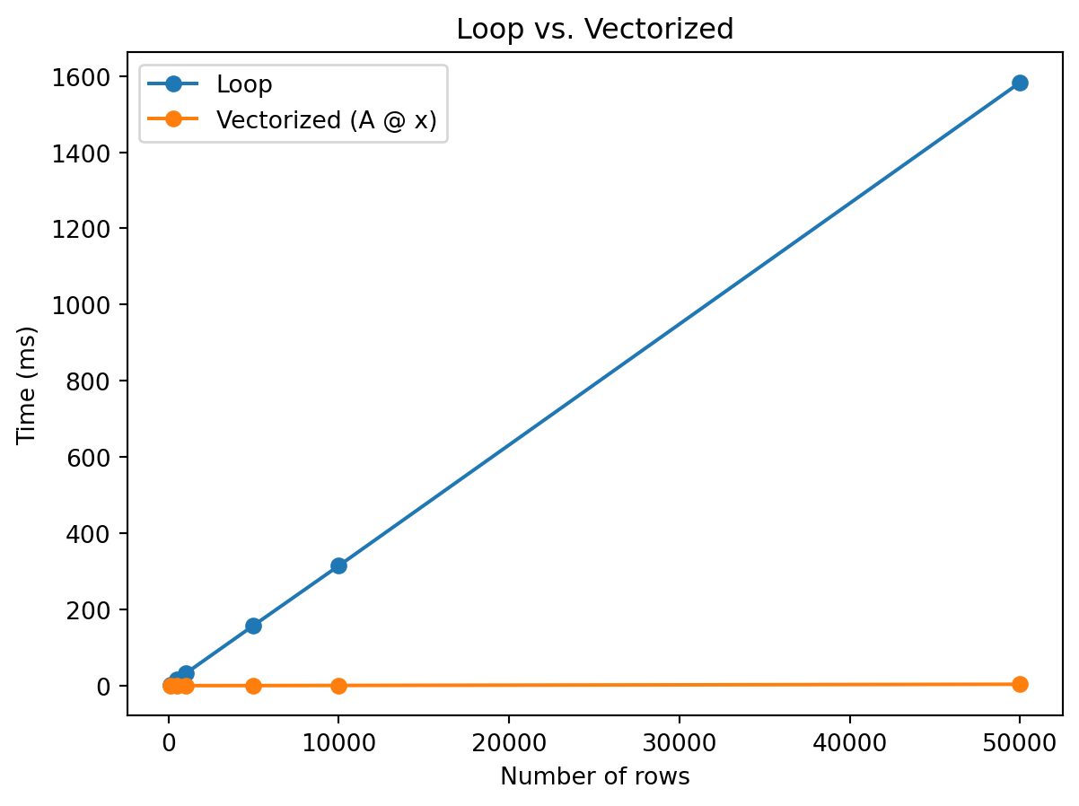

The lesson is simple: whenever you find yourself writing a loop that computes dot products one at a time, there’s probably a single matrix multiply that does the same thing. Writing A @ x instead of a nested loop isn’t just cleaner notation—it’s orders of magnitude faster.

6 Worked Example: State-Contingent Payoffs

Everything in this reference—matrix multiplication, solving systems, rank, determinants—comes together in a classic finance problem: figuring out what your portfolio pays in different future scenarios, and working backward from a desired payoff to find the portfolio that delivers it.

The setup is simple. Suppose the economy can end up in one of \(S\) possible states next period—say recession, normal, or boom. You don’t know which state will occur, but you know what each asset pays in each state. A stock might pay a lot in a boom and nothing in a recession; a bond pays the same regardless; gold does well in bad times and poorly in good times. The question is: given a portfolio of these assets, what do you receive in each state? And: if you want a specific payoff profile across states, what portfolio do you need?

We organize the payoffs in a matrix \(\mathbf{D}\) with \(S\) rows (one per state) and \(N\) columns (one per asset). Entry \(D_{sn}\) is the dollar payoff of one unit of asset \(n\) in state \(s\). Your portfolio positions are a vector \(\boldsymbol{\theta} \in \mathbb{R}^N\), where \(\theta_n\) is the number of units you hold of asset \(n\). The payoff in each state is:

\[\text{payoff vector} = \mathbf{D}\boldsymbol{\theta}\]

Each entry of \(\mathbf{D}\boldsymbol{\theta}\) is the dot product of one row of \(\mathbf{D}\) (one state’s payoffs across all assets) with your position vector—exactly the batched-dot-product idea from earlier.

6.1 Complete markets: \(N = S\)

Consider 3 states and 3 risky assets with the following dollar payoffs per unit held:

	Stock	Gold	Real Estate
Recession	$0	$2	$1
Normal	$1	$1	$3
Boom	$3	$0	$2

The stock pays nothing in a recession and \(\$3\) in a boom—classic equity risk. Gold is the opposite: \(\$2\) in a recession, nothing in a boom (flight to safety). Real estate does best in normal times (\(\$3\)) when the economy is stable, and is weaker in both extremes. All three assets are risky—none has the same payoff in every state. The payoff matrix is:

\[\mathbf{D} = \begin{bmatrix} 0 & 2 & 1 \\ 1 & 1 & 3 \\ 3 & 0 & 2 \end{bmatrix}\]

The forward problem: what does my portfolio pay? Suppose you hold \[\boldsymbol{\theta} = \begin{bmatrix} 4 \\ 3 \\ 2 \end{bmatrix}\] —4 units of stock, 3 units of gold, 2 units of real estate. Your payoff in each state is \(\mathbf{D}\boldsymbol{\theta}\), which is three dot products: one per state.

Recession (row 1): \(0(4) + 2(3) + 1(2) = 0 + 6 + 2 = 8\).

Normal (row 2): \(1(4) + 1(3) + 3(2) = 4 + 3 + 6 = 13\).

Boom (row 3): \(3(4) + 0(3) + 2(2) = 12 + 0 + 4 = 16\).

So \[\mathbf{D}\boldsymbol{\theta} = \begin{bmatrix} 8 \\ 13 \\ 16 \end{bmatrix}\] —you receive \(\$8\) in a recession, \(\$13\) in normal times, and \(\$16\) in a boom. In code:

D = np.array([[0, 2, 1],
              [1, 1, 3],
              [3, 0, 2]])
theta = np.array([4, 3, 2])

payoff = D @ theta
print(f"Payoff in each state: {payoff}")

Payoff in each state: [ 8 13 16]

The math and the code compute the same three dot products.

The inverse problem: what portfolio gives me a target payoff? Now suppose you want a specific payoff: \(\$8\) in recession, \(\$13\) in normal, \(\$16\) in boom. What positions \(\boldsymbol{\theta}\) do you need? This means solving \(\mathbf{D}\boldsymbol{\theta} = \mathbf{b}\) where \[\mathbf{b} = \begin{bmatrix} 8 \\ 13 \\ 16 \end{bmatrix}.\] Written out as equations:

\[\begin{align*} 0\theta_1 + 2\theta_2 + 1\theta_3 &= 8 \\ 1\theta_1 + 1\theta_2 + 3\theta_3 &= 13 \\ 3\theta_1 + 0\theta_2 + 2\theta_3 &= 16 \end{align*}\]

We can solve this by hand using substitution. The first equation gives \(\theta_3 = 8 - 2\theta_2\). Substituting into the second: \(\theta_1 + \theta_2 + 3(8 - 2\theta_2) = 13\), so \(\theta_1 + \theta_2 + 24 - 6\theta_2 = 13\), which gives \(\theta_1 = 5\theta_2 - 11\). Substituting both into the third: \(3(5\theta_2 - 11) + 2(8 - 2\theta_2) = 16\), so \(15\theta_2 - 33 + 16 - 4\theta_2 = 16\), giving \(11\theta_2 = 33\), so \(\theta_2 = 3\). Back-substituting: \(\theta_1 = 5(3) - 11 = 4\) and \(\theta_3 = 8 - 2(3) = 2\). The answer is \[\boldsymbol{\theta} = \begin{bmatrix} 4 \\ 3 \\ 2 \end{bmatrix}\] —exactly the portfolio we started with. Or we can skip the algebra and use np.linalg.solve:

b = np.array([8, 13, 16])

theta_solved = np.linalg.solve(D, b)
print(f"Required positions: {theta_solved}")

# Verify
print(f"D @ theta = {D @ theta_solved}")

Required positions: [4. 3. 2.]
D @ theta = [ 8. 13. 16.]

This works because \(\mathbf{D}\) is \(3 \times 3\) (square) and has full rank. Let’s confirm: \(\det(\mathbf{D}) = 0(1 \cdot 2 - 3 \cdot 0) - 2(1 \cdot 2 - 3 \cdot 3) + 1(1 \cdot 0 - 1 \cdot 3) = 0 - 2(-7) + (-3) = 11\). Non-zero determinant, full rank, the inverse exists:

print(f"det(D) = {np.linalg.det(D):.0f}")
print(f"rank(D) = {np.linalg.matrix_rank(D)}")

det(D) = 11
rank(D) = 3

With \(N = S\) and full rank, we can replicate any target payoff. Want more in booms and less in recessions? Solve with a different \(\mathbf{b}\). Want a risk-free payoff—the same amount in every state? Solve with \[\mathbf{b} = \begin{bmatrix} 100 \\ 100 \\ 100 \end{bmatrix}.\] Even though none of the three assets is individually risk-free, a combination of them can be:

# Replicate a risk-free payoff of $100 in every state
b_riskfree = np.array([100, 100, 100])
theta_rf = np.linalg.solve(D, b_riskfree)
print(f"To get $100 in every state: {np.round(theta_rf, 2)}")
print(f"Verify: {np.round(D @ theta_rf, 10)}")

To get $100 in every state: [27.27 45.45  9.09]
Verify: [100. 100. 100.]

Every payoff vector has a unique portfolio that delivers it. This is what finance theory calls complete markets: there are enough independent assets to span every possible payoff pattern across states.

6.2 When an asset isn’t really “new”

What does “independent” mean here? Suppose we replace real estate with a REIT whose payoff happens to be \[\begin{bmatrix} 2 \\ 2 \\ 3 \end{bmatrix}.\] Compare that to the payoff of holding 1 unit of stock plus 1 unit of gold: \[\begin{bmatrix} 0 \\ 1 \\ 3 \end{bmatrix} + \begin{bmatrix} 2 \\ 1 \\ 0 \end{bmatrix} = \begin{bmatrix} 2 \\ 2 \\ 3 \end{bmatrix}.\] The REIT’s payoff is just a portfolio of stock and gold. It looks like a third asset, but it carries no new information—it’s repackaging exposures you already have.

In linear algebra terms, the REIT’s column is a linear combination of the other two columns. The payoff matrix \[\mathbf{D}_{\text{bad}} = \begin{bmatrix} 0 & 2 & 2 \\ 1 & 1 & 2 \\ 3 & 0 & 3 \end{bmatrix}\] has rank 2, not 3—and its determinant is zero:

D_bad = np.array([[0, 2, 2],
                  [1, 1, 2],
                  [3, 0, 3]])

print(f"det(D_bad) = {np.linalg.det(D_bad):.0f}")
print(f"rank(D_bad) = {np.linalg.matrix_rank(D_bad)}")

det(D_bad) = 0
rank(D_bad) = 2

Even though you have 3 assets and 3 states (\(N = S\)), the market is not complete. One asset is redundant—it’s just a portfolio of the others—so you effectively have only 2 independent instruments. You can’t solve \(\mathbf{D}_{\text{bad}}\boldsymbol{\theta} = \mathbf{b}\) for arbitrary \(\mathbf{b}\) because the matrix isn’t invertible. This is why rank matters: it tells you how many genuinely different assets you have, regardless of how many are listed. The determinant being zero is the numerical signal that at least one asset is redundant.

6.3 Incomplete markets: \(N < S\)

Now suppose real estate isn’t available—you only have the stock and gold. The payoff matrix shrinks to \(3 \times 2\):

\[\mathbf{D}_2 = \begin{bmatrix} 0 & 2 \\ 1 & 1 \\ 3 & 0 \end{bmatrix}\]

This matrix is not square—3 rows and 2 columns—so it cannot be inverted. With only 2 assets, you can’t replicate every possible 3-state payoff. There aren’t enough instruments.

What payoffs can you reach? Any achievable payoff is a combination of the two asset columns: \[\theta_1\begin{bmatrix} 0 \\ 1 \\ 3 \end{bmatrix} + \theta_2\begin{bmatrix} 2 \\ 1 \\ 0 \end{bmatrix} = \begin{bmatrix} 2\theta_2 \\ \theta_1 + \theta_2 \\ 3\theta_1 \end{bmatrix}.\] There are only two free parameters (\(\theta_1\) and \(\theta_2\)) but three payoff entries. Once you choose \(\theta_1\) and \(\theta_2\), all three states are locked in. You can’t independently target recession, normal, and boom—choosing any two pins down the third.

To see this concretely, suppose you want recession \(= 8\) and boom \(= 16\). From the formula above, recession \(= 2\theta_2\) gives \(\theta_2 = 4\), and boom \(= 3\theta_1\) gives \(\theta_1 = 16/3\). But then the normal payoff is forced: \(\theta_1 + \theta_2 = 16/3 + 4 = 9.33\). If you wanted normal \(= 13\), you’re out of luck—there’s no portfolio of just stock and gold that delivers \([8, 13, 16]\).

D2 = np.array([[0, 2],
               [1, 1],
               [3, 0]])

b = np.array([8, 13, 16])

print(f"D2 shape: {D2.shape} -- not square, can't use np.linalg.solve")
print(f"Rank of D2: {np.linalg.matrix_rank(D2)}")
print(f"Normal payoff required for [8, ?, 16]: {16/3 + 8/2:.2f}")
print(f"We wanted 13 -- not achievable")

D2 shape: (3, 2) -- not square, can't use np.linalg.solve
Rank of D2: 2
Normal payoff required for [8, ?, 16]: 9.33
We wanted 13 -- not achievable

The rank of \(\mathbf{D}_2\) is 2—both columns are genuinely different—but rank 2 in a 3-state world means you can only span a 2-dimensional subset of all possible payoff patterns. The achievable payoffs satisfy a constraint (here: \(\text{normal} = \text{boom}/3 + \text{recession}/2\)), and anything outside that constraint is out of reach.

We can still find achievable targets. With \(\theta_1 = 4\) and \(\theta_2 = 3\): recession \(= 2(3) = 6\), normal \(= 4 + 3 = 7\), boom \(= 3(4) = 12\). The payoff \[\begin{bmatrix} 6 \\ 7 \\ 12 \end{bmatrix}\] is achievable. And for the unreachable target \[\begin{bmatrix} 8 \\ 13 \\ 16 \end{bmatrix},\] np.linalg.lstsq finds the closest approximation—but it won’t match exactly:

# Achievable target
theta_ok = np.array([4, 3])
print(f"Achievable: {D2 @ theta_ok}")

# Unreachable target -- best approximation
theta_approx, _, _, _ = np.linalg.lstsq(D2, b, rcond=None)
payoff_approx = D2 @ theta_approx
print(f"\nTarget:      {b}")
print(f"Best approx: {np.round(payoff_approx, 2)}")
print(f"Error:       {np.round(payoff_approx - b, 2)}")

Achievable: [ 6  7 12]

Target:      [ 8 13 16]
Best approx: [ 9.35 10.31 16.9 ]
Error:       [ 1.35 -2.69  0.9 ]

This is the difference between \(N = S\) (complete markets) and \(N < S\) (incomplete markets), stated entirely in linear algebra terms. When \(\mathbf{D}\) is square with full rank, \(\mathbf{D}\boldsymbol{\theta} = \mathbf{b}\) has a unique solution for every \(\mathbf{b}\). When \(\mathbf{D}\) has fewer columns than rows, the system is overdetermined—more equations than unknowns—and most targets have no exact solution. And even when \(N = S\), if one asset is just a portfolio of the others (rank \(< N\)), you’re effectively in the same situation: the determinant is zero, the matrix can’t be inverted, and some payoffs are unreachable.

7 Summary

The throughline of this reference is that matrices batch linear operations. A single dot product computes one predicted return, one portfolio payoff, one state-contingent value. A matrix multiply computes many of them at once. That’s what \(\hat{\mathbf{y}} = \mathbf{X}\boldsymbol{\beta}\) does in OLS (one prediction per observation), and what \(\mathbf{D}\boldsymbol{\theta}\) does in state pricing (one payoff per state).

The machinery around this—transpose, determinant, rank, inverse—exists to answer the reverse question: given an outcome you want, can you find the inputs that produce it? In OLS, that means finding the \(\boldsymbol{\beta}\) that best fits the data, which requires inverting \(\mathbf{X}^\top\mathbf{X}\). In state pricing, that means finding the portfolio \(\boldsymbol{\theta}\) that delivers a target payoff, which requires inverting the payoff matrix \(\mathbf{D}\).

Whether the inverse exists comes down to rank and determinant, and both have direct financial meaning. A payoff matrix that isn’t full rank means one of your assets is redundant—it’s just a repackaged combination of things you already hold. A near-singular \(\mathbf{X}^\top\mathbf{X}\) in regression means your features are nearly collinear, so the model can’t tell which one is actually driving the outcome. In both cases, the determinant is close to zero, the inverse is unstable or nonexistent, and the system can’t give you a unique answer.

In finance, this matters for risk allocation. If your market is incomplete (\(N < S\), or \(N = S\) but with redundant assets), there are payoff profiles you simply cannot construct—risks you cannot hedge, no matter how you trade. The rank of \(\mathbf{D}\) tells you how many independent risk exposures you can actually control. Full rank means you can target any payoff across states; less than full rank means some risks are locked together, and choosing your exposure to one forces your exposure to another. The linear algebra doesn’t just describe the constraint—it is the constraint.

Translating math to code

Operation	Math	NumPy
Dot product	\(\mathbf{x}^\top\mathbf{y}\)	x @ y
Matrix multiply	\(\mathbf{A}\mathbf{B}\)	A @ B
Transpose	\(\mathbf{A}^\top\)	A.T
Transpose of a product	\((\mathbf{A}\mathbf{B})^\top = \mathbf{B}^\top\mathbf{A}^\top\)	(A @ B).T = B.T @ A.T
Identity	\(\mathbf{I}_n\)	np.eye(n)
Determinant	\(\det(\mathbf{A})\)	np.linalg.det(A)
Rank	\(\text{rank}(\mathbf{A})\)	np.linalg.matrix_rank(A)
Solve \(\mathbf{A}\mathbf{x} = \mathbf{b}\)	\(\mathbf{x} = \mathbf{A}^{-1}\mathbf{b}\)	np.linalg.solve(A, b)
OLS coefficients	\(\hat{\boldsymbol{\beta}} = (\mathbf{X}^\top\mathbf{X})^{-1}\mathbf{X}^\top\mathbf{y}\)	np.linalg.solve(X.T @ X, X.T @ y)